四川大学 信号与系统课件
- 格式:pps
- 大小:2.59 MB
- 文档页数:81


《信号与系统》课件讲义一、内容描述首先我们将从信号的基本概念开始,大家都知道,无论是听音乐、看电视还是打电话,背后都离不开信号的存在。
那么什么是信号呢?信号有哪些种类?我们又如何描述它们呢?这一部分我们会带领大家走进信号的世界,一起探索信号的奥秘。
接下来我们将探讨信号与系统之间的关系,信号在系统中是如何传输、处理和变换的?不同的系统对信号有何影响?我们将通过具体的例子和模型,帮助大家理解这个复杂的过程。
此外我们还会深入学习信号的数学描述方法,虽然这部分内容可能会有些难度,但我们会尽量使用通俗易懂的语言,帮助大家更好地理解。
通过这部分的学习,我们将学会如何对信号进行量化分析,从而更好地理解和应用信号。
我们将探讨信号处理的一些基本方法和技术,如何对信号进行滤波、调制、解调等处理?这些处理技术在实际中有哪些应用?我们将通过实例和实践,帮助大家掌握这些基本方法和技术。
1. 介绍信号与系统的基本概念及其重要性首先什么是信号?简单来说信号就像是我们生活中的各种信息传达方式,想象一下当你用手机给朋友发一条短信,这条信息就是一个信号,它传递了你的意图和情感。
在更广泛的层面上,信号可以是任何形式的波动或变化,比如声音、光线、电流等。
它们都有一个共同特点,那就是携带了某种信息。
这些信息可能是我们想要传达的话语,也可能是自然界中的物理变化。
而系统则是接收和处理这些信号的装置或过程,它像是一个加工厂,将接收到的信号进行加工处理,然后输出我们想要的结果。
比如收音机就是一个系统,它接收无线电信号并转换成声音让我们听到。
这样描述下来,你会发现信号和系统真的是无处不在。
无论是在学习还是在日常生活中都能见到他们的影子,他们对现代通信、计算机技术的发展都有着不可替代的作用。
因此我们也需要对这一概念进行透彻的了解与学习才能更好地服务于相关领域为社会贡献力量!2. 简述本课程的学习目标和主要内容《信号与系统》这门课程无论是对于通信工程、电子工程还是计算机领域的学生来说,都是一门极其重要的基础课程。
Ch1. Signals and Systems SIGNALS and SYSTEMS信号与系统任课老师:罗伟E-mail: teacherluowei@Ch1. Signals and Systems •本“信号与系统”课程所讨论的主要内容是:描述确定信号与线性时不变系统的基本数学方法和分析确定信号通过线性时不变系统的基本数学方法。
信号与系统四川大学电气信息工程学院2012年春(64学时)序言•要求本课程注册学生应具备:1.进行复数运算和多项式运算的能力。
2.微积分学和求解常系数常微分方程的基础知识。
3.电路、电子电路、电工测量技术的基本理论与实践。
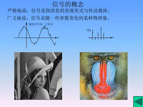
Ch1. Signals and Systems1SIGNALS AND SYSTEMS信号与系统Ch1. Signals and Systems Main content :1.Continuous-Time and Discrete-Time Signals(连续时间与离散时间信号)2.Transformations of the IndependentVariable(自变量的变换)3.Exponential and Sinusoidal Signals(指数信号与正弦信号)4.The Unit Impulse and Unit StepFunctions(单位冲激与单位阶跃函数)5.Continuous-Time and Discrete-TimeSystems (连续时间与离散时间系统)6.Basic System Properties(基本系统性质)1.1 CONTINUOUS-TIME AND DISCRETE-TIME SIGNALS (p1)1.1.1 Examples and Mathematical Representation (p1) (举例与数学表示)•Signals: physical phenomena or physicalquantities, which change with time or space.•Functions of one or more independent variables. example: x(t)Figure 1.1 (p2)A simple RC circuit.A speech signalFigure 1.3 (p2) “Should we chase” 这句话的鸟鸣声的时域波形,其幅值是时间的一元函数心电图——幅值是时间的一元函数A pictureFigure 1.4 (p3) 一幅黑白(monochrome)照片可的函数是是像素的位置 :图片上 B},G ,R { ),( C n m ),(n m CContinuous-time and Discrete-time Signals(连续时间与离散时间信号)•continuous-time signals’ independent variable is continuous : x(t)(p3)•对一切时间t (除有限个不连续点外) 都有确定的函数值,这类信号就称为连续时间信号,简称连续信号。
•discrete-time signals are defined only at discrete times (only for integer values of the independent variable) : x[n] (p4)•仅在不连续的瞬间(仅在自变量的整数值上)有确定函数值Representing Signals Graphically0x (t)tFigure 1.7(p5)Graphical representations of (a)continuous-time and (b)discrete-time signals.(a)-2x [-1]x [0]x [4]-4-3-1012345x [n]n(b)1.1.2Signal Energy and Power (p5)(信号能量与功率))(1)()()(2t v Rt i t v t p ==dt t v Rdt t p t t t t ⎰⎰=2121)(1)(2dt t v Rt t dt t p t t t t t t ⎰⎰-=-2121)(11)(121212(p5), (1.1)(p6), (1.2)(p6), (1.3)The average power isThe instantaneous power isThe total energy isIf v (t )and i (t )are,respectively,the voltage and current across a resistor with resistance R ,thenSignal Energy and PowerA. Continuous-Time SignalInstantaneous Power: 22)( or )()(t x t x t p =Energy over t 1≤t ≤t 2:⎰⎰=2121)()(2t t t t dtt x dt t p Total Energy:⎰-∞→∞=T TT dtt x E )(2lim Average Power:⎰-∞→∞=T TT dtt x TP )(212lim(p6),(1.4)(p6),(1.6)(p7),(1.8)B. Discrete-Time SignalInstantaneous Power: Energy over n 1≤n ≤n 2:Total Energy:Average Power:22][or ][][n x n x n p =∑==21][2n n n n xE ∑∞-∞=∞=n n x E ][2∑-=∞→∞+=NNn N n x N P ][1212lim(p6),(1.5)(p6),(1.7)(p6),(1.9)With these definitions, we can identify threeimportant classes of signals:1,01()0,t x t other≤≤⎧=⎨⎩1E ∞=A.Finite Energy Signal :+∞<=⎰+∞∞-dt t x E )(2+∞<=∑+∞-∞=n n xE ][2( P →0 )Example :(p7)P =B.Finite Power Signal :21[]21lim NN n NP x n N →∞=-=<+∞+∑⎰-∞→+∞<=T T T dt t x T P )(212lim ( E →∞)Example :(p7)[]4x n =C. Signals with neither finite total energy nor finite average powerE ∞=∞16P ∞=()x t t=,E =∞P =∞Example :(p7)1.2TRANSFORMATIONS OF THE INDEPENDENT VARIABLE (p7)(自变量的变换) 1.2.1Examples of Transformations of the Independent Variable(p8)(自变量变换举例)(1) Time ShiftRight shift: x(t-t0) x[n-n0] (Delay)Left shift : x(t+t0) x[n+n0] (Advance)当信号经不同路径传输时,所用时间不同,从而产生时移。
如电视图像出现的重影是由于信号传输的时移造成。
Time Shift (Example) Signal TransformationFigure 1.8 (p8) x[n] and x[n-n] with n>0.Figure 1.9 (p9) x(t-t0) and x(t-t0) with t0<0.(2) Time Reversalx(-t)or x[-n] : Reflection of x(t) or x[n] Figure 1.10 (p9) x[n] Figure 1.11 (p9) x(t)(3) Time Scalingx(at) or x[an]( a>0 )Stretch if a<1Compressed if a>1如录像带慢放时,信号被展宽;快放时,信号被压缩;倒放时,则信号被反褶。
Figure 1.12 (p9)Continuous-time signalsrelated by time scaling.Example 1.1c (complementary)Given a signalx(-t/3+2), shown in Fig. (a), draw the graph of x(t).012t(a)x (-t/3+2)1-2/3-1/301x (t +2)x (t/3+2)1-2-101x (t )1x(-t/3) -6-5-401x(t/3)045604/35/321x(t)012 t(a)x(-t/3+2)11.2.2Periodic Signals(p11)(周期信号)在较长时间内(严格地说,无始无终)每隔一定时间T(或整数N)按相同规律重复变化的信号叫周期信号。
For a continuous-time signal x(t)x(t)=x(t+mT),(m=0,+1,-1,+2,-2,……)(p11,1.11) for all values of t.For a discrete-time signal x[n]x[n]=x[n+mN],(m=0,+1,-1,+2,-2,……)(p12,1.12) for all values of n.In this case,we say that x(t)(x[n])is periodic with Fundamental Period T(N).Examples of periodic signals: sin, cos ,etc.with their fundamental period (基波周期) Figure1.14(p12)A continuous-time period signal.N0=3Example 1.2c (complementary)Determine the fundamental period of the signal x(t)=2cos(10πt+1)-sin(4πt-1).From trigonometry,we know that the fundamental period of cos(10πt+1)is T1=1/5,and sin(4πt-1)is T2=1/2.What about the fundamental period of x(t)? The answer is if there is a rational T,and it is the lowest common multiple of T1and T2,then we say that x(t)is periodic with fundamental period T,or else,x(t)is aperiodic.For the x(t) in this example, the lowest common multiple of 0.2 and 0.5 is unit 1, and it is rational,1.2.3 Even and Odd Signals (p13) (偶信号与奇信号) Even signal: x(-t) = x(t) (p13, 1.14)x[-n]= x[n] (p13, 1.15)Odd signal : x(-t)= -x(t) (p13, 1.16)x[-n]= -x[n] (p13, 1.17)x (t ) = E v {x (t )} + O d {x (t )})]()([21)()}({t x t x t x t x Od o --==]}[][{21][]}[{n x n x n x n x Ev e -+==]}[][{1][]}[{n x n x n x n x Od o --==or:)]()([21)()}({t x t x t x t x Ev e -+==even part of x (t ) odd part of x (t )Even-Odd Decomposition:(p14, 1.18) (p14, 1.19)Example 1.3c (complementary)Even-Odd DecompositionCh1. Signals and Systems 例2.例1:-2210-111-1)(e t x)(o t x tt 0-1-21212)(t x t1.3 EXPONENTIAL AND SINUSOIDAL SIGNALS (p14)(指数信号与正弦信号)1.3.1Continuous-time Complex Exponential andSinusoidal Signals(p15)(连续时间复指数信号与正弦信号) A. Real Exponential Signals (p15)x(t)= C e at( C, a are real value) (p15, 1.20)a >0 a <0Figure1.19(p15)Continuous-time real exponentialB. Periodic Complex Exponential andSinusoidal Signals (p16)(a) x (t ) = e j ω0t (p16, 1.21)(b) x (t ) = Acos(ω0t +φ) (p16, 1.25)All x (t )satisfy for x (t ) = x (t +T ), and T =2π/ ω0, so x (t )is periodic.Euler’s Relation (欧拉关系):e j ω0t =cos ω0t + jsin ω0t (p17, 1.26)and cos ω0t = (e j ω0t +e -j ω0t ) / 2sin ω0t = (e j ω0t -e -j ω0t ) / 2jt j j t j j e e A e e A t A 00)cos(ωφωφφω--+=+We also have (p17, 1.27)C. General Complex Exponential Signals (p20)x (t ) = C e at , in which C = |C |e j θ, a = r + j ω0,so)sin(||)cos(||||||)(00)(00θωθωθωωθ+++===+t e C j t e C ee C ee e C t x rt rt t j rt t j rt j For r=0, the real and imaginary parts of x(t) are sinusoidal; For r>0(r<0), they correspond to sinusoidal signals multiplied by a growing (decaying) exponetial.(p20, 1.43)The dashed curve is the envelope (包络) for the (a)Growing sinusoidal signal ,,r >0;(b)decaying sinusoid ,,r <0.)cos()(0θω+=t Ce t x rt )cos()(0θω+=t Ce t x rt Figure 1.23(p21)Continuous-time complex exponential signals.1.3.2 Discrete-time Complex Exponential and Sinusoidal Signals (p21) (离散时间复指数信号与正弦信号)A. Real Exponential Signals (p22)Figure 1.24 (p23)Discrete-time RealExponential Signalx[n] = Cαn:(a)α>1;(b) 0<α<1;(c) -1<α<0;(d) α<-1.B. Sinusoidal Signals (p22)Discrete-time Complexexponential:x[n]=e jω0n=cosω0n+jsinω0n(p20, 1.43)Figure 1.25 (p24)Discrete-timesinusoidal signal:x[n] = cos(ω0n+φ).C. General Complex Exponential Signals (p24) Complex Exponential Signal:x[n]= Cαnin which C= |C| e jθ, α= |α|e jω0(polar form,极坐标) ,thenx[n]=|C| |α|n cos(ω0n+ θ)+j|C| |α|n sin(ω0n+ θ)(p25, 1.50)(a) Growing sinusoidal sequence(b) Decaying sinusoidal sequence1>α1<αFigure 1.26(p25)Complex Exponential Signals.1.3.3 Periodicity Properties of Discrete-time Complex Exponentials (p25) (离散时间复指数序列的周期性质)Sampling:Discrete-time signals have three majordifferences from its continuous-time partner.n j n t t j ee 00ωω−−→−=Are they the same?No!For e j ω0t ,it has two properties: (p26)A.The larger the magnitude of ω0,the higher is the rate of oscillation in the signal;B.e j ω0t is periodic for any value of ω0.A. For discrete-time complex exponentialsignals, we need to consider a frequencyinterval of 2π. (p26) (在考虑离散时间复指数时,仅需要在某一个2π间隔内选择即可)n j n j n j n j e e e e 0002)2(ωπωπω==+Thus, e j ω0 n and e j(ω0 +2 π) n are the same signals. πωππω<≤-<≤00 or ,20e j ω0 n 不具备随ω0在数值上的增加而不断增加其振荡速率的特性!当ω0从0开始增加,其振荡速率愈来愈快,直到ω0= π,达到最大,若继续增加ω0,其振荡速率就下降,直到ω0= 2π时,又得到与ω0=0时同样的效果(常数序列).(p26, 1.51)Lowest oscillation rate: Highest oscillation rate:,4,2,0ππω±±=,3,ππω±±=Figure 1.27(p27)Discrete-time SinusoidalB. Periodicity of e jω0n (p26)Continuous-time: e jω0t,T=2π/ω0Discrete-time: e jω0n,N=?Calculate period:By definition: e jω0n=e jω0(n+N) (p26, 1.53)thus e jω0N= 1(p26, 1.54) orω0N=2πm (p26, 1.55) So N=2πm/ω0with interger N (p28, 1.58) Condition of periodicity: 2π/ω0is rational.若2π/ω为一有理数,e jω0n就是周期的,否则就不是周期的.C. Finite number of distinct harmonics (p29),2,1,0 ,][)(2±±==k en n jk k N πφFor a periodic signal with fundamentalperiod of N ,][][)(2)())((222n e e e e n k n jk n j n jk n N k j N k N N N φφππππ====++There are only N distinct periodic exponentials for discrete-time signals.In the Continuous-time case,all of the harmonicallyrelated complex exponentials 2(),0,1,2,Tjk t e k π=±± (p29, 1.60) (p30, 1.61)1.4THE UNIT IMPULSE AND UNIT STEP FUNCTIONS (p30)(单位冲激与单位阶跃函数)1.4.1The Discrete-Time Unit Impulse and Unit Step Sequences (p30)(离散时间单位脉冲与单位阶跃序列)Unit Sample (Impulse):⎩⎨⎧=≠=0,10,0][n n n δ(p30, 1.63) Figure 1.28(p30)Discrete-time unit impulse (sample).Unit Step Function:⎩⎨⎧≥<=0,10,0][n n n u (p30, 1.64) Figure 1.29(p31)Discrete-timeunit stepsequence.Relationship between unit sample and unit step sequencethe unit sample is the first difference of the unit step sequence]1[][][--=n u n u n δ the unit step sequence is the running sum of the unitsample ∑-∞==nm m n u ][][δ∑∞=-=0][][k k n n u δor0,[]1,n k n k n kδ≠⎧-=⎨=here (p31, 1.65) (p31, 1.66)(p31, 1.67)][]0[][][n x n n x δδ=][][][][k n k x k n n x -=-δδ∑+∞-∞=-=k k n k x n x ][][][δwrite any discrete-time signal in terms of delayed unit sample as Sampling Property of Unit Sample(p32, 1.68)(p32, 1.69)Unit Step Function :1.4.2The Continuous-Time Unit Step and Unit Impulse Functions (p32)(离散时间单位脉冲与单位阶跃序列)⎩⎨⎧><=0,10,0)(t t t u (p32, 1.70)Figure 1.32(p33)Continuous-time unit step function.Unit Impulse Function:⎰∞+∞-=⎩⎨⎧=∞≠=1)(and 0,0,0)(dt t t t t δδFigure 1.35(p34)Continuous-time unit impulse.。