Non-overshooting PI control of variable-speed motor drives with sliding perturbation observers

Goodman Manufacturing Company, L.P .2550 North Loop West, Suite 400Houston, TX -or-The Furnace Twinning Kit (FTK) provides the means for two (2) Amana ® brand or Goodman ® brand gas furnaces containing an Integrated Ignition control to operate at the same time from a single thermostat. The two furnaces to be “twinned” must be exactly the same model with their circulating air blowers set to deliver the same air flow at the same time. The furnaces may deliver different CFMs in the cooling mode, if appropriate. THIS KIT CANNOT BE USED TO CONTROL MORE THAN TWO (2) FURNACES. When properly installed, these furnaces will achieve the operational and performance specifications described in the installation instructions. For items not covered in this manual, follow the installation instructions shipped with the furnaces.This Twinning Kit Installation Instruction is divided into five sections. Section I deals with furnace opening sizes, recommended filter sizes and maximum CFM per furnace. Section II details the installation of the twinning kit. Section III details the sequence of operation. Section IV provides checks and possible repair procedures. Section V provides a point-to-point wiring diagram.Bottom ReturnIn most cases, bottom return air to both upflow furnaces will be more practical. When bottom return air is used, the furnaces should be set as close together (0 to 3 inches) as is practical. This separation distance is variable, depending upon the needs of the particular job.See furnace specification sheet for furnace opening sizes, recommended filter sizes, and maximum CFM per furnace.Side Return (One Return per Furnace)This is applicable only for the upflow models with less than five tons of airflow.P REFERRED M ETHODPlace the furnaces close together and install a return air drop to the out-side of each furnace (Figure 1).Figure 1 - [Preferred Method] Single-Side Return Per Furnace SideCutouts are 14" x 23" (All Furnaces)A LTERNATE M ETHODThe alternate method is used when the installer is forced to use one re-turn for two furnaces (Figure 2). The maximum required spacing between the furnaces is 30 inches apart (approximately 28 x 24 return trunk duct).F URNACE T WINNING K ITI NSTALLATION I NSTRUCTIONSNOTE: NOT FOR USE WITH TWO-STAGE VARIABLE SPEED FURNACES OR WITH 2-STAGE CONDENSING UNITS.SECTION 1 GENERAL INFORMATIONIt is very important to properly size ductwork and to supply appropriate filters for your furnaces. There are four possible ductwork configurations for twinning your furnaces:•Bottom Return•Side Return - One Return per Furnace •Two Side Returns •Top Return IMPORTANT NOTE: Back return duct installations to furnaces are NOT permitted. Back return installations constrict airflow which leads to poor performance and equipment damage. Back return installations are con-sidered improper installation and will void warranty coverage.GENERAL NOTES•Maximum CFMs are limited by a maximum filter velocity of 600 feet per minute, or by circulator high speed at 0.5 inches External Static Pressure (ESP) (whichever CFM is lower). THIS REQUIRES A HIGH VELOCITY FILTER. THROWAWAY FILTERS MUST NOT BE USED.If using anything other than a permanent high velocity filter, consult filter manufacturer recommendations for maximum allowable veloc-ity.•Actual CFM at the job should be established by carefully setting the furnace input and measuring the temperature rise. The ESP/CFM Tables in the furnace specification sheets and installation manuals are based on side return(s) for a single furnace. For twinned installa-tions - especially those with bottom return - the relationship between ESP and CFM may be different. The most accurate way to estimate airflow on twinned installations is to use temperature rise:CFM =BTUH Input1.085 x (Supply Air Temperature - Return Air Temperature)•Cooling CFM should be 350 to 450 CFM per nominal ton of cooling capacity. Heating CFM must produce a temperature rise within the range(s) specified on the furnace nameplate.©1998-2006 Goodman Manufacturing Company, L.P.Effective: March 2006Part No. IO-656Printed in USAFigure 2 - [Alternate Method] Single-Side Return per FurnaceSide Cutouts are 14" x 23" Furnaces are 30" ApartTwo Side ReturnsTwo side returns per furnace is ordinarily used when only 8 or 10 tons of cooling are required and where a bottom return is not practical. The fur-naces should be from 24 to 30 inches apart. Two side returns are applicableonly for upflow models with five tons of airflow.Figure 3 - Two Side Returns Per Furnace SideCutouts are 14" x 23 " (All Furnaces)Top ReturnWhen counterflow furnaces are twinned, the return air must enter through the top of the furnace.See the furnace specification sheet for minimum plenum height and maximum CFMs per furnace. Filter racks areincluded with the furnaces.Figure 4 - Twinned Counterflow Furnaces"A" = Minimum Plenum Height Furnaces from 0 to 30" ApartSECTION II TWINING KIT INSTALLATIONThis Installation Kit includes:ABBTwinning Kit Item Quantity DescriptionA 1Johnson Controls Y88FA-3 Twinning ControlB 2Fan Sensor Field Supplied Material 2 - #6 Screws 3/4" long18 Gauge 5-Wire ConductorTools Required 1/4" Nut Driver Drill3/32" Drill BitSmall Regular (Common) ScrewdriverBefore Installing the Twinning KitThere are important items which must be determined before installing the twinning kit. Read all of these instructions before you begin install-ing either furnace.Continuous Fan OperationFurnaces that are twinned using this kit cannot be setup for heating-cooling-continuous fan speed operation. When the furnaces are set for continuous fan operation, it will be at the cooling fan speed. This applies to models using 50A50-288, 50A55-288, 50T55-288, 50A65-288 controls only. Models using 50A55-289 or 50A65-289 controls are set for continu-ous fan operation at the heating fan speed.Condensate DisposalWhen installing condensing furnaces, be sure to plan for adequate con-densate drainage. This is especially important on counterflow installations. Follow the condensate disposal piping directions shipped with the fur-nace.Unit WiringThis kit allows the furnaces to be placed a maximum of five feet apart. Wire routing between furnaces is the same for any type furnace being installed. IMPORTANT NOTE: Any excess wires must be routed and secured to prevent becoming entangled in either blower or damaged by either set of burners.Kit Installation1.Disconnect all electrical power to unit.2.Find a location for mounting the twinning control. The side of thereturn section of the furnace cabinet or on the return air duct would be adequate locations.NOTE: The control should be mounted in a location that allows ac-cess to the terminals for wiring and servicing and keeps wire lengths to a minimum.3.Drill two holes according to the following illustration (Figure 5).2.05" 4" 6.76"6.20"4.56"Figure 5Mounting Hole Locationsing two #6 3/4-inch long screws (field-supplied), mount the twin-ning control vertically with the label right side up. Ensure the screws are located in opposite corners of the control. Do not over tighten the screws. DO NOT expose the control to water or temperatures below -40°F or above 120°F.5.Designate one of the furnaces as furnace #1 and the other as fur-nace #2.6.Connect furnace #1’s ignition control thermostat connectors: C, R, W,Y, and G to an 18 gauge 5-wire thermostat cable.7.Route the cable up through the blower deck and out the thermostatwire hole on the side of the cabinet. Connect the wires to the corresponding terminals on the furnace #1 section of the twinning control.8.Repeat steps 6 and 7 for furnace #2. Fan Sensor Wiring Installation1.Remove the backing paper from the adhesive backed Fan Sensor andattach to the #1 furnace control mounting plate next to the furnace control module.2.Route the three wire cable along the same path as the thermostatwiring to the twinning control.3.Connect the three wires to the corresponding FAN/LED SENSOR IN-PUTS on the furnace #1 section of the twinning control. The cable can be cut to a convenient length.4.Locate any two fan motor speed tap wires (red, black, blue, or or-ange), even if they are unused.IMPORTANT NOTE: To prevent damage to the fan sensor do not choose the WHITE “neutral” lead wire.5.Connect one of the two motor leads to one of the black wires from thefan sensor with the “Y” terminal provided. Repeat this step for the other fan lead.6.Connect the “Y” terminal to the original location of the motor speed tapwire.Note: The connector should be taped if the motor speed tap wire is not connected to the furnace control module.7.The two white wires attached to the fan sensor must be taped orwire nuts added to prevent accidental connections. These white wires have no connections.8.Repeat steps 1 through 7 for furnace #2.Thermostat Wiring InstallationImportant Note: The system thermostat that controls the conditioned space should not have a current draw higher than 25 milliamps.1.The system thermostat connects to the 6-terminal strip on the oppo-site side of the Twinning Control from the furnace inputs. The control allows the use of a two stage heating and cooling thermostat. If a single stage heating or cooling thermostat is used the W1 and W2 (1 stage heating) or Y1 and Y2 (1 stage cooling) must be jumped to-gether. For thermostats that require a “common” connection a “C”terminal is provided.2.The heat anticipator in the room thermostat must be correctly adjustedto obtain the proper number of heating cycles per hour and to prevent the room temperature from “overshooting” the room thermostat set-ting. Heat anticipator must be set at 0.16 amps.SECTION III SEQUENCE OF OPERATIONSingle Stage ThermostatOn a system call for heat a relay closes both blower (R-G) circuits, pow-ering the blowers of both furnaces (continuous fan speed). One second later, relays close the heating (R-W) circuits of both furnaces. In 30 or 45 seconds after the furnaces fire, the blowers will switch to the heating speed. When the call for heat is satisfied at the thermostat, both (R-W) circuits will immediately open. Following approximately a 65 second delay, the fan (R-G) circuits will open.For cooling operation, the sequence is identical but with the R-Y circuits activated.NOTE: In the heating mode, if the furnace control module blower off timing is longer than the Twinning Control's 65 seconds, the blower(s) will con-tinue to operate in the heating speed until the furnace control module blower off delay is satisfied.Two-Stage ThermostatOn a first stage call for heat, a relay will close both blower (R-G) circuits as in the single stage operation. One second later, a relay will close the heating circuit (R-W) of furnace #2 only. In 30 or 45 seconds after the furnaces light, the blower of furnace #2 will switch to the heating speed. When the call for heat is satisfied, the (R-W) circuit will open and the 65 second Twinning Control fan off delay begins. The furnace #2 blower will operate in the heating speed until the furnace control module blower off delay is satisfied, then the blower will switch to the continuous fan speed.NOTE: If the furnace control blower off delay is longer than the 65 second Twinning Control off delay, the Twinning Control will turn off the blowers.The blower for furnace #1 will shut off, and since the blower on furnace #2 is still running, the blower for furnace #1 will reenergize in the continuous fan speed. This process will continue until the furnace control blower off timing is satisfied and both blowers are running in the continuous fan speed. The Twinning Control will then simultaneously turn off both blowers.To prevent this operation, set both furnace's heat off delay time to 60seconds.On the next stage 1 call for heat, furnace #1 is signaled to heat. This sequence alternates on successive cycles balancing run times on the furnaces.If a stage 2 (W2) call for heat is received at any time W1 is activated the R-W circuit of the non-firing furnace closes.If both stages energize or deenergize simultaneously, operation is identical to single stage operation above.Two stage cooling is analogous to staged heating but activates the R-Y cir-cuits. The blowers will have a 65 second off delay in the cooling speed.Abnormal ConditionsIf only one blower is sensed “ON” for more than four seconds while a thermostat input is present, both furnaces will deenergize and the on-board LEDs are activated. This lockout condition can be reset by turning the thermostat to the OFF position or by turning the power OFF then back ON for both furnaces for at least one second and returning to the desired function. If, when no thermostat input is present, only a single blower is sensed, the blower circuits (R-G) close to both furnaces for 65 seconds and then open. If the unbalanced condition (one blower sensed), still ex-ists, the sequence repeats.Diagnostic LED Flash SequenceThe on-board LED activates with a blower failure on furnace 1, 2, or both.If the furnace blower failure is on furnace 1, the LED will flash once with a two-second off interval between flashes.If the furnace blower failure is on furnace 2, the LED will flash twice with a two-second off interval between flash sequences.If the furnace blower failure is on both furnaces, the LED will flash three times with a two-second off interval between flash sequences.SECTION IV CHECKOUT AND REPAIRSStartup ProcedureRefer to the Installation Instructions provided with the furnace for proper operation and startup procedures after installing the twinning control. If that information is not available, follow these instructions to ensure all components function properly:1.With the gas and thermostat off, turn ON power to the furnaces.2.Turn the thermostat to a high setting and verify that both ignition con-trols go through the operating sequence to a shutoff condition.Note: The burners will not light because the gas is off.3.Turn OFF the thermostat.4.Turn ON the gas and purge gas lines of all air.5.Check for gas leaks with a soap solution.6.Turn the thermostat to a high setting and verify successful ignition and a normal run condition for at least three minutes.7.Do a leak check on all pipe joints downstream of the gas valve with a soap solution.8.Turn the thermostat down for at least 30 seconds and then back up again. Verify successful ignition at least three times before leaving the installation.Repairs and ReplacementDo not attempt field repairs. Use only an exact or factory recommended replacement control.SECTION V POINT-TO-POINT WIRING DIAGRAM。

PACKAGING INFORMATIONOrderable Device Status(1)Package Type Package DrawingPins Package Qty Eco Plan (2)Lead/Ball Finish MSL Peak Temp (3)5962-7700801VCA ACTIVE CDIP J 141None A42SNPB Level-NC-NC-NC 5962-87739012A ACTIVE LCCC FK 201None POST-PLATE Level-NC-NC-NC5962-8773901CA ACTIVE CDIP J 141None A42SNPB Level-NC-NC-NC 5962-8773901DA ACTIVE CFP W 141None A42SNPB Level-NC-NC-NC 77008012A ACTIVE LCCC FK 201None POST-PLATE Level-NC-NC-NC7700801CA ACTIVE CDIP J 141None A42SNPB Level-NC-NC-NC 7700801DA ACTIVE CFP W 141None A42SNPB Level-NC-NC-NC JM38510/11201BCAACTIVE CDIP J 141None A42SNPB Level-NC-NC-NC LM139AD ACTIVE SOIC D 1450None CU NIPDAU Level-3-245C-168HR LM139ADR ACTIVE SOIC D 142500Pb-Free (RoHS)CU NIPDAULevel-2-250C-1YEAR/Level-1-235C-UNLIM LM139AFKB ACTIVE LCCC FK 201None POST-PLATE Level-NC-NC-NC LM139AJ ACTIVE CDIP J 141None A42SNPB Level-NC-NC-NC LM139AJB ACTIVE CDIP J 141None A42SNPB Level-NC-NC-NC LM139AN OBSOLETE PDIP N 14None Call TI Call TILM139AW ACTIVE CFP W 141None A42SNPB Level-NC-NC-NC LM139AWB ACTIVE CFP W 141None A42SNPB Level-NC-NC-NC LM139D ACTIVE SOIC D 1450None CU NIPDAU Level-1-220C-UNLIM LM139DR ACTIVE SOIC D 142500None CU NIPDAU Level-1-220C-UNLIM LM139FKB ACTIVE LCCC FK 201None POST-PLATE Level-NC-NC-NCLM139J ACTIVE CDIP J 141None A42SNPB Level-NC-NC-NC LM139JB ACTIVE CDIP J 141None A42SNPB Level-NC-NC-NC LM139N OBSOLETE PDIP N 14None Call TI Call TILM139W ACTIVE CFP W 141None A42SNPB Level-NC-NC-NC LM139WB ACTIVE CFP W 141None A42SNPB Level-NC-NC-NC LM239AD ACTIVE SOIC D 1450Pb-Free (RoHS)CU NIPDAU Level-2-260C-1YEAR/Level-1-235C-UNLIM LM239ADR ACTIVE SOIC D 142500Pb-Free (RoHS)CU NIPDAU Level-2-260C-1YEAR/Level-1-235C-UNLIM LM239AN OBSOLETE PDIP N 14None Call TI Call TILM239D ACTIVE SOIC D 1450Pb-Free (RoHS)CU NIPDAU Level-2-260C-1YEAR/Level-1-235C-UNLIM LM239DR ACTIVE SOIC D 142500Pb-Free (RoHS)CU NIPDAU Level-2-260C-1YEAR/Level-1-235C-UNLIM LM239N ACTIVE PDIP N 1425Pb-Free (RoHS)CU NIPDAU Level-NC-NC-NC LM239PW ACTIVE TSSOP PW 1490Pb-Free (RoHS)CU NIPDAU Level-1-250C-UNLIM LM239PWR ACTIVE TSSOP PW 142000Pb-Free (RoHS)CU NIPDAU Level-1-250C-UNLIM LM2901AVQDR ACTIVE SOIC D 142500Pb-Free (RoHS)CU NIPDAU Level-2-250C-1YEAR/Level-1-235C-UNLIM LM2901AVQPWRACTIVE TSSOP PW 142000None CU NIPDAU Level-1-250C-UNLIM LM2901DACTIVESOICD1450Pb-Free (RoHS)CU NIPDAULevel-2-260C-1YEAR/Level-1-235C-UNLIM18-Feb-2005Orderable Device Status(1)PackageType PackageDrawing Pins PackageQtyEco Plan(2)Lead/Ball Finish MSL Peak Temp(3)LM2901DR ACTIVE SOIC D142500Pb-Free(RoHS)CU NIPDAU Level-2-260C-1YEAR/Level-1-235C-UNLIMLM2901N ACTIVE PDIP N1425Pb-Free(RoHS)CU NIPDAU Level-NC-NC-NCLM2901NSR ACTIVE SO NS142000Pb-Free(RoHS)CU NIPDAU Level-2-260C-1YEAR/Level-1-235C-UNLIMLM2901PW ACTIVE TSSOP PW1490Pb-Free(RoHS)CU NIPDAU Level-1-250C-UNLIM LM2901PWLE OBSOLETE TSSOP PW14None Call TI Call TILM2901PWR ACTIVE TSSOP PW142000Pb-Free(RoHS)CU NIPDAU Level-1-250C-UNLIM LM2901QD OBSOLETE SOIC D14None Call TI Call TILM2901QN OBSOLETE PDIP N14None Call TI Call TILM2901VQDR ACTIVE SOIC D142500Pb-Free(RoHS)CU NIPDAU Level-2-250C-1YEAR/Level-1-235C-UNLIMLM2901VQPWR ACTIVE TSSOP PW142000None CU NIPDAU Level-1-250C-UNLIMLM339AD ACTIVE SOIC D1450Pb-Free(RoHS)CU NIPDAU Level-2-260C-1YEAR/Level-1-235C-UNLIMLM339ADBR ACTIVE SSOP DB142000Pb-Free(RoHS)CU NIPDAU Level-2-260C-1YEAR/Level-1-235C-UNLIMLM339ADR ACTIVE SOIC D142500Pb-Free(RoHS)CU NIPDAU Level-2-260C-1YEAR/Level-1-235C-UNLIMLM339AN ACTIVE PDIP N1425Pb-Free(RoHS)CU NIPDAU Level-NC-NC-NCLM339ANSR ACTIVE SO NS142000Pb-Free(RoHS)CU NIPDAU Level-2-260C-1YEAR/Level-1-235C-UNLIMLM339APW ACTIVE TSSOP PW1490Pb-Free(RoHS)CU NIPDAU Level-1-250C-UNLIMLM339APWR ACTIVE TSSOP PW142000Pb-Free(RoHS)CU NIPDAU Level-1-250C-UNLIMLM339D ACTIVE SOIC D1450Pb-Free(RoHS)CU NIPDAU Level-2-260C-1YEAR/Level-1-235C-UNLIMLM339DBLE OBSOLETE SSOP DB14None Call TI Call TILM339DBR ACTIVE SSOP DB142000Pb-Free(RoHS)CU NIPDAU Level-2-260C-1YEAR/Level-1-235C-UNLIMLM339DR ACTIVE SOIC D142500Pb-Free(RoHS)CU NIPDAU Level-2-260C-1YEAR/Level-1-235C-UNLIMLM339N ACTIVE PDIP N1425Pb-Free(RoHS)CU NIPDAU Level-NC-NC-NC LM339NSLE OBSOLETE SO NS14None Call TI Call TILM339NSR ACTIVE SO NS142000Pb-Free(RoHS)CU NIPDAU Level-2-260C-1YEAR/Level-1-235C-UNLIMLM339PW ACTIVE TSSOP PW1490Pb-Free(RoHS)CU NIPDAU Level-1-250C-UNLIM LM339PWLE OBSOLETE TSSOP PW14None Call TI Call TILM339PWR ACTIVE TSSOP PW142000Pb-Free(RoHS)CU NIPDAU Level-1-250C-UNLIM LM339Y OBSOLETE0None Call TI Call TI(1)The marketing status values are defined as follows:18-Feb-2005ACTIVE:Product device recommended for new designs.LIFEBUY:TI has announced that the device will be discontinued,and a lifetime-buy period is in effect.NRND:Not recommended for new designs.Device is in production to support existing customers,but TI does not recommend using this part in a new design.PREVIEW:Device has been announced but is not in production.Samples may or may not be available.OBSOLETE:TI has discontinued the production of the device.(2)Eco Plan -May not be currently available -please check /productcontent for the latest availability information and additional product content details.None:Not yet available Lead (Pb-Free).Pb-Free (RoHS):TI's terms "Lead-Free"or "Pb-Free"mean semiconductor products that are compatible with the current RoHS requirements for all 6substances,including the requirement that lead not exceed 0.1%by weight in homogeneous materials.Where designed to be soldered at high temperatures,TI Pb-Free products are suitable for use in specified lead-free processes.Green (RoHS &no Sb/Br):TI defines "Green"to mean "Pb-Free"and in addition,uses package materials that do not contain halogens,including bromine (Br)or antimony (Sb)above 0.1%of total product weight.(3)MSL,Peak Temp.--The Moisture Sensitivity Level rating according to the JEDECindustry standard classifications,and peak solder temperature.Important Information and Disclaimer:The information provided on this page represents TI's knowledge and belief as of the date that it is provided.TI bases its knowledge and belief on information provided by third parties,and makes no representation or warranty as to the accuracy of such information.Efforts are underway to better integrate information from third parties.TI has taken and continues to take reasonable steps to provide representative and accurate information but may not have conducted destructive testing or chemical analysis on incoming materials and chemicals.TI and TI suppliers consider certain information to be proprietary,and thus CAS numbers and other limited information may not be available for release.In no event shall TI's liability arising out of such information exceed the total purchase price of the TI part(s)at issue in this document sold by TI to Customer on an annualbasis.18-Feb-2005IMPORTANT NOTICETexas Instruments Incorporated and its subsidiaries (TI) reserve the right to make corrections, modifications, enhancements, improvements, and other changes to its products and services at any time and to discontinue any product or service without notice. Customers should obtain the latest relevant information before placing orders and should verify that such information is current and complete. All products are sold subject to TI’s terms and conditions of sale supplied at the time of order acknowledgment.TI warrants performance of its hardware products to the specifications applicable at the time of sale in accordance with TI’s standard warranty. T esting and other quality control techniques are used to the extent TI deems necessary to support this warranty. Except where mandated by government requirements, testing of all parameters of each product is not necessarily performed.TI assumes no liability for applications assistance or customer product design. Customers are responsible for their products and applications using TI components. T o minimize the risks associated with customer products and applications, customers should provide adequate design and operating safeguards.TI does not warrant or represent that any license, either express or implied, is granted under any TI patent right, copyright, mask work right, or other TI intellectual property right relating to any combination, machine, or process in which TI products or services are used. Information published by TI regarding third-party products or services does not constitute a license from TI to use such products or services or a warranty or endorsement thereof. Use of such information may require a license from a third party under the patents or other intellectual property of the third party, or a license from TI under the patents or other intellectual property of TI.Reproduction of information in TI data books or data sheets is permissible only if reproduction is without alteration and is accompanied by all associated warranties, conditions, limitations, and notices. Reproduction of this information with alteration is an unfair and deceptive business practice. TI is not responsible or liable for such altered documentation.Resale of TI products or services with statements different from or beyond the parameters stated by TI for that product or service voids all express and any implied warranties for the associated TI product or service and is an unfair and deceptive business practice. TI is not responsible or liable for any such statements. Following are URLs where you can obtain information on other Texas Instruments products and application solutions:Products ApplicationsAmplifiers Audio /audioData Converters Automotive /automotiveDSP Broadband /broadbandInterface Digital Control /digitalcontrolLogic Military /militaryPower Mgmt Optical Networking /opticalnetwork Microcontrollers Security /securityTelephony /telephonyVideo & Imaging /videoWireless /wirelessMailing Address:Texas InstrumentsPost Office Box 655303 Dallas, Texas 75265Copyright 2005, Texas Instruments Incorporated。

PID controller免费的百科全书Jump to: navigation, search跳转到:导航搜索A block diagram of a PID controller一个PID控制器的框图A proportional比例–integral积分–derivative 微分controller (PID controller) is a generic control loop feedback mechanism (controller) widely used in industrial control systems– a PID is the most commonly used feedback controller. A PID controller calculates an "error" value as the difference between a measured process variable and a desired setpoint. The controller attempts to minimize the error by adjusting the process control inputs.The PID controller calculation (algorithm) involves three separate constant parameters, and is accordingly sometimes called three-term control: the proportional, the integral and derivative values, denoted P,I, and D.Heuristically, these values can be interpreted in terms of time: P depends on the present error, I on the accumulation of past errors, and D is a prediction of future errors, based on current rate of change.[1] The weighted sum of these three actions is used to adjust the process via a control element such as the position of a control valve, or the power supplied to a heating element.In the absence of knowledge of the underlying process, a PID controller has historically been considered to be the best controller.[2] By tuning the three parameters in the PID controller algorithm, the controller can provide control action designed for specific process requirements. The response of the controller can be described in terms of the responsiveness of the controller to an error, the degree to which the controller overshoots the setpoint and the degree of system oscillation. Note that the use of the PID algorithm for control does not guarantee optimal control of the system or system stability.Some applications may require using only one or two actions to provide the appropriate system control. This is achieved by setting the other parameters to zero. A PID controller will be called a PI, PD, P or Icontroller in the absence of the respective control actions. PI controllers are fairly common, since derivative action is sensitive to measurement noise, whereas the absence of an integral term may prevent the system from reaching its target value due to the control action.Contents[hide]∙ 1 Control loop basics∙ 2 PID controller theoryo 2.1 Proportional term2.1.1 Droopo 2.2 Integral termo 2.3 Derivative term∙ 3 Loop tuningo 3.1 Stabilityo 3.2 Optimum behavioro 3.3 Overview of methodso 3.4 Manual tuningo 3.5 Ziegler–Nichols methodo 3.6 PID tuning software∙ 4 Modifications to the PID algorithm∙ 5 History∙ 6 Limitations of PID controlo 6.1 Linearityo 6.2 Noise in derivative∙7 Improvementso7.1 Feed-forwardo7.2 Other improvements∙8 Cascade control∙9 Physical implementation of PID control∙10 Alternative nomenclature and PID formso10.1 Ideal versus standard PID formo10.2 Basing derivative action on PVo10.3 Basing proportional action on PVo10.4 Laplace form of the PID controllero10.5 PID Pole Zero Cancellationo10.6 Series/interacting formo10.7 Discrete implementationo10.8 Pseudocode∙11 PI controller∙12 See also∙13 References∙14 External linkso14.1 PID tutorialso14.2 Special topics and PID control applications [edit] Control loop basics基本控制回路Further information更多信息: Control system控制系统A familiar example of a control loop is the action taken when adjusting hot and cold faucets (valves) to maintain the water at a desired temperature. This typically involves the mixing of two process streams, the hot and cold water. The person touches the water to sense or measure its temperature. Based on this feedback they perform a control action to adjust the hot and cold water valves until the process temperature stabilizes at the desired value.The sensed water temperature is the process variable or process value (PV). The desired temperature is called the setpoint (SP). The input to the process (the water valve position) is called the manipulated variable (MV). The difference between the temperature measurement and the set point is the error (e) and quantifies whether the water is too hot or too cold and by how much.After measuring the temperature (PV), and then calculating the error, the controller decides when to change the tap position (MV) and by how much. When the controller first turns the valve on, it may turn the hot valve only slightly if warm water is desired, or it may open the valve all the way if very hot water is desired. This is an example of a simple proportional control. In the event that hot water does not arrive quickly, the controller may try to speed-up the process by opening up the hot water valve more-and-more as time goes by. This is an example of an integral control.Making a change that is too large when the error is small is equivalent to a high gain controller and will lead to overshoot. If the controller were to repeatedly make changes that were too large and repeatedly overshoot the target, the output would oscillate around the setpoint in either a constant, growing, or decaying sinusoid. If the oscillations increase with time then the system is unstable, whereas if they decrease the system is stable. If the oscillations remain at a constant magnitude the system is marginally stable.In the interest of achieving a gradual convergence at the desired temperature (SP), the controller may wish to damp the anticipated future oscillations. So in order to compensate for this effect, the controller may elect to temper its adjustments. This can be thought of as a derivative control method.If a controller starts from a stable state at zero error (PV = SP), then further changes by the controller will be in response to changes in other measured or unmeasured inputs to the process that impact on the process, and hence on the PV. Variables that impact on the process other than the MV are known as disturbances. Generally controllers are used to reject disturbances and/or implement setpoint changes. Changes in feedwater temperature constitute a disturbance to the faucet temperature control process.In theory, a controller can be used to control any process which has a measurable output (PV), a known ideal value for that output (SP) and an input to the process (MV) that will affect the relevant PV. Controllers are used in industry to regulate temperature, pressure, flow rate, chemical composition, speed and practically every other variable for which a measurement exists.[edit] PID controller theoryThis section describes the parallel or non-interacting form of the PID controller. For other forms please see the section Alternative nomenclature and PID forms.The PID control scheme is named after its three correcting terms, whose sum constitutes the manipulated variable (MV). The proportional, integral, and derivative terms are summed to calculate the output of the PIDcontroller. Defining as the controller output, the final form of the PID algorithm is:where: Proportional gain, a tuning parameter: Integral gain, a tuning parameter: Derivative gain, a tuning parameter: Error: Time or instantaneous time (the present) [edit] Proportional termPlot of PV vs time, for three values of Kp (Kiand Kdheld constant)The proportional term makes a change to the output that is proportional to the current error value. The proportional response can be adjusted by multiplying the error by a constant K p, called the proportional gain.The proportional term is given by:A high proportional gain results in a large change in the output for a given change in the error. If the proportional gain is too high, the system can become unstable (see the section on loop tuning). In contrast, a small gain results in a small output response to a large input error, and a less responsive or less sensitive controller. If the proportional gain is too low, the control action may be too small when responding to system disturbances. Tuning theory and industrial practice indicate that the proportional term should contribute the bulk of the output change.[citation needed][edit] DroopA pure proportional controller will not always settle at its target value, but may retain a steady-state error. Specifically, drift in the absence of control, such as cooling of a furnace towards room temperature, biases a pure proportional controller. If the drift is downwards, as in cooling, then the bias will be below the set point, hence the term "droop".Droop is proportional to the process gain and inversely proportional to proportional gain. Specifically the steady-state error is given by:Droop is an inherent defect of purely proportional control. Droop may be mitigated by adding a compensating bias term (setting the setpoint above the true desired value), or corrected by adding an integral term.[edit] Integral termPlot of PV vs time, for three values of Ki (Kpand Kdheld constant)The contribution from the integral term is proportional to both the magnitude of the error and the duration of the error. The integral in a PID controller is the sum of the instantaneous error over time and gives the accumulated offset that should have been corrected previously. Theaccumulated error is then multiplied by the integral gain () and added to the controller output.The integral term is given by:The integral term accelerates the movement of the process towards setpoint and eliminates the residual steady-state error that occurs with a pure proportional controller. However, since the integral term responds to accumulated errors from the past, it can cause the present value to overshoot the setpoint value (see the section on loop tuning).[edit] Derivative termPlot of PV vs time, for three values of Kd (Kpand Kiheld constant)The derivative of the process error is calculated by determining the slope of the error over time and multiplying this rate of change by thederivative gain . The magnitude of the contribution of the derivative term to the overall control action is termed the derivative gain, . The derivative term is given by:The derivative term slows the rate of change of the controller output. Derivative control is used to reduce the magnitude of the overshoot produced by the integral component and improve the combinedcontroller-process stability. However, the derivative term slows thetransient response of the controller. Also, differentiation of a signal amplifies noise and thus this term in the controller is highly sensitive to noise in the error term, and can cause a process to become unstable if the noise and the derivative gain are sufficiently large. Hence an approximation to a differentiator with a limited bandwidth is more commonly used. Such a circuit is known as a phase-lead compensator.[edit] Loop tuningTuning a control loop is the adjustment of its control parameters (proportional band/gain, integral gain/reset, derivative gain/rate) to the optimum values for the desired control response. Stability (bounded oscillation) is a basic requirement, but beyond that, different systems have different behavior, different applications have different requirements, and requirements may conflict with one another.PID tuning is a difficult problem, even though there are only three parameters and in principle is simple to describe, because it must satisfy complex criteria within the limitations of PID control. There are accordingly various methods for loop tuning, and more sophisticated techniques are the subject of patents; this section describes some traditional manual methods for loop tuning.Designing and tuning a PID controller appears to be conceptually intuitive, but can be hard in practice, if multiple (and often conflicting) objectives such as short transient and high stability are to be achieved. Usually, initial designs need to be adjusted repeatedly through computer simulations until the closed-loop system performs or compromises as desired.Some processes have a degree of non-linearity and so parameters that work well at full-load conditions don't work when the process is starting up from no-load; this can be corrected by gain scheduling (using different parameters in different operating regions). PID controllers often provide acceptable control using default tunings, but performance can generally be improved by careful tuning, and performance may be unacceptable with poor tuning.[edit] StabilityIf the PID controller parameters (the gains of the proportional, integral and derivative terms) are chosen incorrectly, the controlled process input can be unstable, i.e., its output diverges, with or withoutoscillation, and is limited only by saturation or mechanical breakage. Instability is caused by excess gain, particularly in the presence of significant lag.Generally, stabilization of response is required and the process must not oscillate for any combination of process conditions and setpoints, though sometimes marginal stability (bounded oscillation) is acceptable or desired.[citation needed][edit] Optimum behaviorThe optimum behavior on a process change or setpoint change varies depending on the application.Two basic requirements are regulation (disturbance rejection – staying at a given setpoint) and command tracking(implementing setpoint changes) –these refer to how well the controlled variable tracks the desired value. Specific criteria for command tracking include rise time and settling time. Some processes must not allow an overshoot of the process variable beyond the setpoint if, for example, this would be unsafe. Other processes must minimize the energy expended in reaching a new setpoint.[edit] Overview of methodsThere are several methods for tuning a PID loop. The most effective methods generally involve the development of some form of process model, then choosing P, I, and D based on the dynamic model parameters. Manual tuning methods can be relatively inefficient, particularly if the loops have response times on the order of minutes or longer.The choice of method will depend largely on whether or not the loop can be taken "offline" for tuning, and the response time of the system. If the system can be taken offline, the best tuning method often involves subjecting the system to a step change in input, measuring the output as a function of time, and using this response to determine the control parameters.Choosing a Tuning MethodMethod Advantages DisadvantagesManual Tuning No math required. Online method. Requires experienced personnel.Ziegler–Nichols Proven Method. Online method. Process upset, sometrial-and-error, veryaggressive tuning.Software Tools Consistent tuning. Online oroffline method. May includevalve and sensor analysis. Allow simulation before downloading. Can support Non-Steady State(NSS) Tuning.Some cost and training involved.Cohen-Coon Good process models. Some math. Offline method. Only good forfirst-order processes.[edit ] Manual tuningIf the system must remain online, one tuning method is to first set and values to zero. Increase the until the output of the loop oscillates, then the should be set to approximately half of that valuefor a "quarter amplitude decay" type response. Then increaseuntil any offset is corrected in sufficient time for the process. However, too muchwill cause instability. Finally, increase , if required, until the loop is acceptably quick to reach its reference after a load disturbance. However, too much will cause excessive response and overshoot. A fast PID loop tuning usually overshoots slightly to reach the setpoint more quickly; however, some systems cannot accept overshoot, in which case an over-damped closed-loop system is required, which will require a setting significantly less than half that of the setting causing oscillation. Effects of increasing a parameter independently Parameter Rise time OvershootSettlingtime Steady-state error Stability [3] Decrease Increase Smallchange DecreaseDegrade Decrease [4] Increase Increase Decrease DegradesignificantlyMinor decrease Minor decrease Minor decrease No effect intheory Improve if small[edit ] Ziegler –Nichols methodFor more details on this topic, see Ziegler –Nichols method .Another heuristic tuning method is formally known asthe Ziegler –Nichols method , introducedbyJohnG.ZieglerandNathaniel B. Nichols in the 1940s. As in the method above, the and gains are first set to zero. TheP gain is increased until it reaches the ultimate gain,, at which the output of the loop starts to oscillate.and the oscillation periodare used to set the gains as shown:Ziegler –Nichols methodControl Type P- - PI-PID These gains apply to the ideal, parallel form of the PID controller. When applied to the standard PID form, the integral and derivative time parameters and are only dependent on the oscillation period . Please see the section "Alternative nomenclature and PID forms ".[edit ] PID tuning softwareMost modern industrial facilities no longer tune loops using the manual calculation methods shown above. Instead, PID tuning and loopoptimization software are used to ensure consistent results. These software packages will gather the data, develop process models, andsuggest optimal tuning. Some software packages can even develop tuning by gathering data from reference changes.Mathematical PID loop tuning induces an impulse in the system, and then uses the controlled system's frequency response to design the PID loop values. In loops with response times of several minutes, mathematical loop tuning is recommended, because trial and error can take days just to find a stable set of loop values. Optimal values are harder to find. Some digital loop controllers offer a self-tuning feature in which very small setpoint changes are sent to the process, allowing the controller itself to calculate optimal tuning values.Other formulas are available to tune the loop according to different performance criteria. Many patented formulas are now embedded within PID tuning software and hardware modules.Advances in automated PID Loop Tuning software also deliver algorithms for tuning PID Loops in a dynamic or Non-Steady State (NSS) scenario. The software will model the dynamics of a process, through a disturbance, and calculate PID control parameters in response.[edit] Modifications to the PID algorithmThe basic PID algorithm presents some challenges in control applications that have been addressed by minor modifications to the PID form.Integral windupFor more details on this topic, see Integral windup.One common problem resulting from the ideal PID implementations is integral windup, where a large change in setpoint occurs (say a positive change) and the integral term accumulates an error larger than the maximal value for the regulation variable (windup), thus the system overshoots and continues to increase as this accumulated error is unwound. This problem can be addressed by:∙Initializing the controller integral to a desired value∙Increasing the setpoint in a suitable ramp∙Disabling the integral function until the PV has entered the controllable region∙Limiting the time period over which the integral error is calculated ∙Preventing the integral term from accumulating above or below pre-determined boundsOvershooting from known disturbancesFor example, a PID loop is used to control the temperature of an electric resistance furnace, the system has stabilized. Now the door is opened and something cold is put into the furnace thetemperature drops below the setpoint. The integral function of the controller tends to compensate this error by introducing another error in the positive direction. This overshoot can be avoided by freezing of the integral function after the opening of the door for the time the control loop typically needs to reheat the furnace. Replacing the integral function by a model based partOften the time-response of the system is approximately known. Then it is an advantage to simulate this time-response with a model and to calculate some unknown parameter from the actual response of the system. If for instance the system is an electrical furnace the response of the difference between furnace temperature and ambient temperature to changes of the electrical power will be similar to that of a simple RC low-pass filter multiplied by an unknownproportional coefficient. The actual electrical power supplied to the furnace is delayed by a low-pass filter to simulate the response of the temperature of the furnace and then the actual temperature minus the ambient temperature is divided by this low-pass filtered electrical power. Then, the result is stabilized by anotherlow-pass filter leading to an estimation of the proportionalcoefficient. With this estimation, it is possible to calculate the required electrical power by dividing the set-point of thetemperature minus the ambient temperature by this coefficient. The result can then be used instead of the integral function. This also achieves a control error of zero in the steady-state, but avoids integral windup and can give a significantly improved controlaction compared to an optimized PID controller. This type ofcontroller does work properly in an open loop situation which causes integral windup with an integral function. This is an advantage if, for example, the heating of a furnace has to be reduced for some time because of the failure of a heating element, or if thecontroller is used as an advisory system to a human operator who may not switch it to closed-loop operation. It may also be useful if the controller is inside a branch of a complex control system that may be temporarily inactive.Many PID loops control a mechanical device (for example, a valve). Mechanical maintenance can be a major cost and wear leads to control degradation in the form of either stiction or a deadband in the mechanical response to an input signal. The rate of mechanical wear is mainly a function of how often a device is activated to make a change. Where wearis a significant concern, the PID loop may have an output deadband to reduce the frequency of activation of the output (valve). This is accomplished by modifying the controller to hold its output steady if the change would be small (within the defined deadband range). The calculated output must leave the deadband before the actual output will change.The proportional and derivative terms can produce excessive movement in the output when a system is subjected to an instantaneous step increase in the error, such as a large setpoint change. In the case of the derivative term, this is due to taking the derivative of the error, which is very large in the case of an instantaneous step change. As a result, some PID algorithms incorporate the following modifications:Derivative of the Process VariableIn this case the PID controller measures the derivative of themeasured process variable (PV), rather than the derivative of the error. This quantity is always continuous (i.e., never has a step change as a result of changed setpoint). For this technique to be effective, the derivative of the PV must have the opposite sign of the derivative of the error, in the case of negative feedbackcontrol.Setpoint rampingIn this modification, the setpoint is gradually moved from its old value to a newly specified value using a linear or first orderdifferential ramp function. This avoids the discontinuity present in a simple step change.Setpoint weightingSetpoint weighting uses different multipliers for the errordepending on which element of the controller it is used in. The error in the integral term must be the true control error to avoidsteady-state control errors. This affects the controller'ssetpoint response. These parameters do not affect the response to load disturbances and measurement noise.[edit] HistoryThis section requires expansion.PID theory developed by observing the action of helmsmen.PID controllers date to 1890s governor design.[2][5] PID controllers were subsequently developed in automatic ship steering. One of the earliest examples of a PID-type controller was developed by Elmer Sperry in 1911,[6] while the first published theoretical analysis of a PID controller was by Russian American engineer Nicolas Minorsky, in (Minorsky 1922). Minorsky was designing automatic steering systems for the US Navy, and based his analysis on observations of a helmsman, observing that the helmsman controlled the ship not only based on the current error, but also on past error and current rate of change;[7]this was then made mathematical by Minorsky. His goal was stability, not general control, which significantly simplified the problem. While proportional control provides stability against small disturbances, it was insufficient for dealing with a steady disturbance, notably a stiff gale (due to droop), which required adding the integral term. Finally, the derivative term was added to improve control.Trials were carried out on the USS New Mexico, with the controller controlling the angular velocity (not angle) of the rudder. PI control yielded sustained yaw (angular error) of ±2°, while adding D yielded yaw of ±1/6°, better than most helmsmen could achieve.[8]The Navy ultimately did not adopt the system, due to resistance by personnel. Similar work was carried out and published by several others in the 1930s.[edit] Limitations of PID controlWhile PID controllers are applicable to many control problems, and often perform satisfactorily without any improvements or even tuning, they can perform poorly in some applications, and do not in general provide optimal control. The fundamental difficulty with PID control is that it is a feed back system, with constant parameters, and no direct knowledge of the process, and thus overall performance is reactive and a compromise –while PID control is the best controller with no model of the process,[2] better performance can be obtained by incorporating a model of the process.The most significant improvement is to incorporate feed-forward control with knowledge about the system, and using the PID only to control error. Alternatively, PIDs can be modified in more minor ways, such as by changing the parameters (either gain scheduling in different use cases or adaptively modifying them based on performance), improving measurement (higher sampling rate, precision, and accuracy, and low-pass filtering if necessary), or cascading multiple PID controllers.PID controllers, when used alone, can give poor performance when the PID loop gains must be reduced so that the control system does not overshoot, oscillate or hunt about the control setpoint value. They also have difficulties in the presence of non-linearities, may trade-off regulation versus response time, do not react to changing process behavior (say, the process changes after it has warmed up), and have lag in responding to large disturbances.[edit] LinearityAnother problem faced with PID controllers is that they are linear, and in particular symmetric. Thus, performance of PID controllers innon-linear systems (such as HVAC systems) is variable. For example, in temperature control, a common use case is active heating (via a heating element) but passive cooling (heating off, but no cooling), so overshoot can only be corrected slowly –it cannot be forced downward. In this case the PID should be tuned to be overdamped, to prevent or reduce overshoot, though this reduces performance (it increases settling time).[edit] Noise in derivativeA problem with the derivative term is that small amounts of measurement or process noise can cause large amounts of change in the output. It is often helpful to filter the measurements with a low-pass filter in order to remove higher-frequency noise components. However, low-pass filtering and derivative control can cancel each other out, so reducing noise by instrumentation is a much better choice. Alternatively, a nonlinear median filter may be used, which improves the filtering efficiency and practical performance.[9]In some case, the differential band can be turned off in many systems with little loss of control. This is equivalent to using the PID controller as a PI controller.。

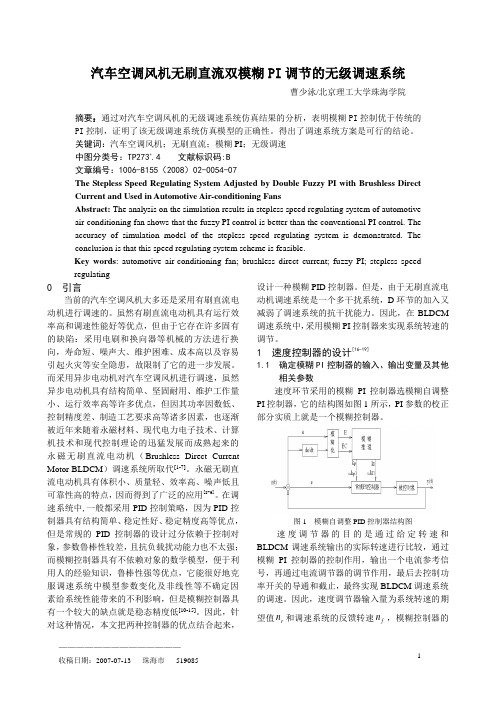
汽车空调风机无刷直流双模糊PI调节的无级调速系统曹少泳/北京理工大学珠海学院摘要：通过对汽车空调风机的无级调速系统仿真结果的分析，表明模糊PI控制优于传统的PI控制，证明了该无级调速系统仿真模型的正确性。

得出了调速系统方案是可行的结论。

关键词：汽车空调风机；无刷直流；模糊PI；无级调速中图分类号：TP273+.4 文献标识码:B文章编号：1006-8155（2008）02-0054-07The Stepless Speed Regulating System Adjusted by Double Fuzzy PI with Brushless Direct Current and Used in Automotive Air-conditioning FansAbstract: The analysis on the simulation results in stepless speed regulating system of automotive air-conditioning fan shows that the fuzzy PI control is better than the conventional PI control. The accuracy of simulation model of the stepless speed regulating system is demonstrated. The conclusion is that this speed regulating system scheme is feasible.Key words: automotive air-conditioning fan; brushless direct current; fuzzy PI; stepless speed regulating0 引言当前的汽车空调风机大多还是采用有刷直流电动机进行调速的。

Offical settlements balance measures the sum of the current account balance plus the (nonofficial)fiancial account balance关键词：balance余额，current account balance经常账户余额，private financial account私人金融帐户官方翻译：官方结算差额等于经常账户余额和私人金融账户余额之和。

通俗翻译：B=CA+FAOvershooting the actual exchang rate then moves slowly back to that long-run rate later is ,in the actual exchange rate overshoots its long-run value and then reverts back toward it关键词：monetary policy货币政策官方翻译：快速大的反应，目前的汇率作为货币政策的变化等消息是所谓的过度。

通俗翻译：政府给个小政策，汇率市场对这个政策的反映过度Sterilized intervention if the authority does take action to prevent the domestic money supply from changing, then the authority is relying only on intervention to defend the fixed rate.关键词：sterilized杀菌使无用，intervention干预，authority官方，take action采取行动，domestic国内的，fixed rate固定汇率官方翻译：官方采取的行动，以防止改变国内货币供应量，官方的干预是为了捍卫固定汇率。

SIMOCRANE integrated STS, GSU Version V3.0These notes take precedence over information in other documents.Please read the notes through carefully because they contain information that it is important for you to know during installation and use of the software.In this version V3.0, the following new features, feature enhancements and feature improvements have been madeSway control functions−New function …Soft Approach“ with consideration of fixed and variable blocked regions in Manual Mode (MAN)−Improving of the function to calculate interpolation points and extending of criterions to start Semi-Automatic Mode (SAM)−Extension of the functional scope of the control bit “START_2D_CALC“−Separated damping factors for acceleration and deceleration (P85, P86, P88, P89)−New parameter (P87) to eliminate the overshooting in positioning process (POS und SAM)−New parameter (P119) for selecting of the lowering point for SAM travel from WS to LS−New parameter (P112, P113) to adapt the trajectory during inclined movement in SAM−Improving of the following error monitoring (E41, E42) for positioning process (POS und SAM) −Expansion of the interface to the higher-level controller (PLC)−New DCC-block “DCC_SCIntPo” to transfer the interpolation points of trajectory to the higher- level controller (PLC)−All camera data will be transferred to the higher-level controller (PLC)−General troubleshooting−Adaption of parameters (Limit values, default value or option)−Extending and improvement of the operation instructions manualsCommissioning and Diagnostic Tool …CeCOMM”−Extending of visualization (limit lines, safety clearance, immersion point…)−Adding the time stamp to the long-time trace−Increasing the number of logger files to 12−New function to calculate the maximum sway deflection−Improvement of the diagram in X/Y-view−Improving of the trace function−Adding a list of all variable signals for trace−TroubleshootingThe Version V3.0 is downwards compatible to the version V 2.1 SP2 HF1. Due to the functional and interface extension, adjustments and new commissioning are required for upgrading. More information about the V2.1 SP2 HF1 refers to the product update for its delivery release:https:///cs/ww/en/view/109750239Contents1. SCOPE OF SUPPLY1.1 DVD1.2 Certificate of License2. NOTES ON INSTALLATION2.1. System requirements2.1.1 Hardware2.1.2 Optional Hardware2.1.3 Software2.2. Installation2.3 Unstalling3. CONSTRAINTS AND FUNCTIONAL RESTRICTIONS1 Scope of Supply1.1 DVDThe DVD contains:The version V3.0 is downwards compatible to the V2.1 SP2 HF1. The software will be put in production and additionally provided for download in internet under ‘Industry Online Support international with Download-ID 109220170, see the following link:https:///cs/ww/en/view/103965095Users can upgrade their application if required. Please pay attention to the preconditions in the operation manual, 07/2019. More information to upgrade your application refer to the FAQhttps:///cs/ww/en/view/109478006Limitation of liabilityThe Software package includes following application examples:•Application example for STS•Application example for GSUThe application example inside the software package are provided free of charge. The customer is granted the non-exclusive, non-transferable, free right to use it. This includes the right to modify the application example, to reproduce it modified or unmodified, and to combine it with the user's own software.All liability, on whatever legal basis, in particular based on errors in the software or the associated documentation or damage resulting from advice, is excluded unless liability is mandatory, for example, due to malice, gross negligence, injury to life, body, or health, due to acceptance of a quality warranty, due to fraudulent concealment of a defect, or due to breach of substantial contractual obligations. This does not imply a reversal of the burden of proof to the detriment of the customer.The customer is furthermore obligated to release SIEMENS AG from any claims of third parties where such claims arise in connection with use of the software by the customer.German law shall apply. The courts of Erlangen shall have exclusive jurisdiction.Safety instructionsSiemens provides products and solutions with industrial security functions that support the secure operation of plants, solutions, machines, equipment and/or networks. They are important components of a holistic industrial security concept. The products and solutions from Siemens are continuously developed with this aspect in mind. Siemens recommends strongly that you regularly check for product updates.For the secure operation of Siemens products and solutions, it is necessary to take suitable preventive action (e.g. cell protection concept) and integrate each component into a holistic, state-of-the-art industrial security concept. Any third-party products that may be in use must also be taken into account. You will find more information about industrial security at: /industrialsecurityConstantly up-to-date information on SIMOCRANE products, product support, FAQs can be found on the Internet: https:///cs/ww/en/ps/200871.2 Certificate of LicenseIn the licensing method used for SIMOTION dependent on the way and number of the runtime components used in the project different licenses must be acquired. The licenses required for a device are assigned to a License key. The license is bound about the serial number of the CF card.The compact flash card (CF card) is not in the scope of supply; a license key must be generated and transferred to the CF card. This will be realized with the help of the enclosed "Certificate of License".Further indications for the license handling will be available in the operating instructions. "SIMOCRANE SC integrated STS, GSU”2 Notes on Installation2.1. System requirementsThe preconditions are a main crane controller system with a PROFIBUS/PROFINET interface as well as continuously controllable drives.Depending on the task to be performed and the environmental conditions, the sway control system can be used with or without a SIMOCRANE CenSOR V2.0 HF3 camera measuring system.The hardware and software required for the camera measuring system must be ordered separately and are not listed here.A version with the necessary hardware components and the required license authority must be available.2.1.1 Hardware• SIMOTION D435-2 DP/PN as of firmware V5.2 SP1 or higher•SINAMICS, as of firmware V5.1.HF1 or higher2.1.2 Optional hardware•SIMOCRANE CenSOR V2.0 HF3•Reflector2.1.3 Software• SIMOTION SCOUT as of Version V5.2 SP1•Optional package Drive Control Chart (DCC) for SIMOTION / SINAMICS as of version V3.1 SP1 •SIMOCRANE Basic Technology Version V3.0•Commissioning and diagnose tool SIMOCRANE CeCOMM ab Version V4.4.2.4•SIMOCRANE SC integrated STS, GSU V3.0•Microsoft Windows 7 or 10•SIMATIC Manager ab V5.62.2. InstallationThe software package contains a setup file. You can use it to install the DCC library "SwayControl." The precondition is that the SIMOTION SCOUT software has been installed and the user is logged onto the PC with administrator rights."Setup_CeCOMM.exe"The installation program leads you step by step through the whole installation process. Installation isperformed as follows:•The SIMATIC Manager and the SCOUT must be closed before the setup is run.•For the procedure for linking the "Sway Control DCC Library" into your SIMOTION user project, see the operating instructions "SIMOCRANE_SC_integrated_STS_GSU_de.pdf" Chapter 5.The software package contains a setup file for the "SIMOCRANE CeCOMM" diagnostics and commissioning tool. The program can run under the WINDOWS 7 or WINDOWS 10 operating system. This requires that the user is logged in the PC with administration rights.Setup_CeCOMM.exeThe installation program guides you through the entire installation process step by step. After installation the diagnostic program will be available under "Windows Start → Programs."2.3UninstallingVia Windows Start →Control panel →Programs, you can uninstall the diagnostics tool installed via setup.3. Constraints and functional restrictionsMethod of operation P140 (3525253)P140 must be left as 0.Function of the P77 (3534325)Leave the parameter P77 with its default value (200).Function of the parameters P149 and P150 (3555469)Leave the parameters P149 and P150 with their default values (0).Function of the P111 (752485)An Adjustment of 0 or 1 for P111 causes no smoothing. Between these values decreasingvalues lead to an increasing smoothing. Values smaller than 0,1 should be avoided. Thesmoothing has no influence to the closed-loop control and effects only the display of the trace in CeCOMM.Workaround: Leave the parameter P111 with its default value (0).P53 Acceleration reduction when hoisting (751425)With values of the parameter P53 < 100 %, unexpected acceleration behaviour of the hoist may occur.Workaround: Parameter P53 must be left with its default value (100%).Warning messages E20 to E27 (1002665)Warning messages E20 to E27 do not work. Functioning of the prelimit switch and limit switchmust be assured in the higher-level control.Target control function (301654)In the case of the hoist and trolley, the target control function results in the target always beingtraveled to with a deviation from P162 or P165 (positioning accuracy). Parameters P163 andP160 must not be less than 0 if the target is to be traveled to without this deviation.Workaround: Do not set parameters P163 and 160 smaller than 0.Stopping a cylinder movement in operation mode “Cylinder jogging”As a result of incorrect Position sensing it may happen that despite correct control according to the operation instructions the movement of the Cylinder cannot be stopped.Workaround: By resetting of the control bit …move“ the cylinders can be stopped ev en in case of incorrect positon sensing (without down ramp).The time-optimal control algorithmus is not used for STS-cranes.Workaround: The time-optimal control algorithmus (P152) should not be used for STS-cranes(P102=1).Operation mode …Cylinder jogging“As a result of incorrect Position measurement it may happen thatDespite correct control according to the operation instructions the movement of the Cylindercannot be stopped.Despite of the selection of only one cylinder more cylinders are moving at the same time.Workaround:By resetting of the control bit …move“ the cylinders can be stopped even in case of incorrectpositon sensing (without down ramp).With an interlock (in PLC) of the state bits …a_out“ up to …d_out“ and …a_in“ up to …d_in“(Zyl inder retract and extend) with the corresponding control bit …a_in_comm“ up to…d_in_comm“ and …a_out_comm“ up to …d_out_comm“ it is possible that only the selectedcylinder is moving.Trolley uncontrolled acceleration (4310214)Trolley uncontrolled acceleration.Abhilfe:Use the delivered new application project.End。

1.Agglomeration economies 联合经济2.Economic interdependence 经济相互依存性w of comparative advantage 比较优势原理4.Autarky 自给自足经济5.Basis for trade 贸易基础plete specialization 完全专业化7.Constant oppor tunity costs 不变机会成本8.Consumption gains 消费者利益9.Exit barriers 退出壁垒10.F ree trade 自由贸易11.G ains from international trade 国际贸易收益12.I ncreasing opportunity costs 机会成本递增13.L abor theory of value 劳动价值理论14.M arginal rate of transformation 边际转换率15.M ercantilists 重商主义16.P artial specialization 部分专业化17.p rice-specie-flow doctrine 价格流转学说18.P rinciple of absolute advantage 绝对优势理论19.P rinciple of comparative advantage 比较优势原理20.P roduction gains 专业化的生产受益21.P roduction possibilities schedule 生产可能性曲线22.T erms of trade 贸易条件23.T rade triangle 贸易三角形24.T rading possibilities line 贸易可能性曲线25.C ommodity terms of trade 商品贸易条件26.C ommunity indifference curve 社会无差异曲线27.I mmiserizing growth 贫困化增长28.i mportance of being unimportant 充当不重要角色的重要性29.i ndifference curve 无差异曲线30.i ndifference map 无差异图31.M arginal rate of substitution 边际替代率32.N o-trade boundary 不贸易边界33.O ffer curve 提供曲线34.O uter limits for the equilibrium terms of trade贸易均衡条件的外部限制35.R egion of mutually beneficial trade 互惠贸易区36.T heory of reciprocal demand 相互需求理论37.B usiness services 商业服务38.D istribution of income 收入分配39.D ynamic comparative advantage 动态比较优势40.E conomies of scale 规模经济41.E nvironmental regulation 环境管制42.F actor-endowment theory 要素禀赋理论43.F actor-price equalization 要素价格均等化44.H eckscher-Ohlin theory 赫克歇尔-奥林理论45.I ndustrial policy 产业政策46.I nterindustry specialization 产业间专业化47.I nterindustry trade 产业间贸易48.I ntraindusty specialization 产业内专业化49.I ntraindusty trade 产业内贸易50.L eontief paradox 里昂惕夫之谜51.P olluter-pays principle 污染者付费原则52.P roduct life cycle theory 产品生命同期理论53.S pecific-factors theory 持定要素理论54.T heory of overlappling demands 需求重叠理论55.T ransportation costs 运输成本56.A d valorem tariff 从价关税57.B eggar-thy-neighbor policy 以邻为壑政策58.B onded warehouse 保税仓库59.C ompound tariff 混合关税60.C onsumer surplus 消费者剩余61.C onsumption effect 消费效益62.C ost-insurance-freight(CIF) valuation 到岸价格63.C ustoms valuation 海关估价64.D eadweight loss 无谓损失65.D omestic revenue effect 国内收入效应66.E ffective tariff rate 有效关税率67.F oreign-trade zone(FTZ) 对外贸易区68.F ree-on-board(FOB)valuation FOB 离岸估价法69.F ree-trade argument 自由贸易理论70.F ree-trade-biased sector 赞成自由贸易部门71.I nfant-industry argument 幼稚产业保护论72.l arge nation 大国73.L evel playing field 公平竞争场74.N ominal tariff rate 名义关税率75.O ffshore-assembly provision(OAP) 境外装配条款76.O ptimum tariff 最优关税77.P roducer surplus 生产者剩余78.P roduction sharing 生产分工79.P rotection-biased sector 赞成贸易保护的部门80.P rotective effect 保护效应81.P rotective tariff 保护关税82.R edistributive effect 再分配效应83.R evenue effect 收入效应84.R evenue tariff 收入关税额85.S cientific tariff 科学关税86.S mall nation 小国87.S pecific tariff 从量关税88.T ariff 关税89.T ariff escalation 关税升级90.T erms-of-trade effect 贸易条件效应91.A ntidumping duty 反倾销税92.B uy-national policies 购买国货政策93.C orporate average fuel economy standards(CAFE)公司平均燃料经济标准94.C ost-based definition of dumping 倾销成本定义95.D omestic content requirement 国内含量条件96.d omestic subsidy 国内补贴97.D umping 倾销98.E xport quota 出口配额99.E xport-revenue effect 出口收入效应100.Export subsidy 出口补贴101.Foreign sourcing 国外外包102.Global quota 全球配额103.Import quota 进口配额104.Margin of dumping 边际倾销105.Nonrestrained suppliers 非限制性供货商106.Nontariff trade barriers(NTBs) 非关税贸易壁垒107.Orderly marketing agreement(OMA) 有序销售协定108.Persistent dumping 持续性倾销109.Predatory dumping 掠夺性倾销110.Price-based definition of dumping 倾销的价格定义111.Selective quota 选择性配额112.Social regulation 社会管制113.Sporadic dumping 偶发性倾销114.Subsidies 补贴115.Tariff-rate quota 关税税率配额116.Trade-diversion effect 贸易转移效应117.Voluntary export restraints(VER) 自愿出口限制modity Credit Corporation(CCC) 商品信用公司119.Countervailing duty 反补贴税120.Economic sanctions 经济制裁121.Escape clause 豁免条款122.Export-import bank 进出口银行123.Fast-trade authority 快速通道权力124.General Agreement on Tariffs and Trade(GATT)关税和贸易总协定125.Intellectual proper ty rights(IPRs) 知识产权126.Kennedy round 肯尼迪回合127.Ministry of international trade and Industry(MITI)国际贸易和产业部128.Most-favored-nation(MFN) clause 最惠国条款129.Normal trade relations 正常贸易关系130.Reciprocal Trade Agreements Act 互惠贸易协定法案131.section301 301条款132.Smoot-Hawley Act 斯母特-郝利法案133.Strategic trade policy 战略性贸易政策134.Tokyo round 东京回合135.Trade adjustment assistance 贸易调整援助136.Trade promotion authority 贸易促进当局137.Trade remedy laws 贸易补偿条款138.Uruguay Round 乌拉圭回合139.Wage insurance 工资保险140.WorldTrade Organization(WTO) 世界贸易组织141.Advanced nations 发达国家142.Buffer stock 缓冲存货143.developing nations 发展中国家144.Cartel 卡特尔145.East Asian tigers 东亚老虎146.Export controls 出口控制147.Export-led growth 出口带动性增长148.Export-oriented policy 出口导向性政策149.Flying-geese pattern of economic growth 经济增长的飞鹅模式150.Generalized system of preference(GSP) 普惠制151.Import substitution 进口替代152.Inter national commodity agreement(ICAs) 国际商品协定153.Multilateral contract 多边合同154.New international economic order 国际经济新秩序anization of Petroleum Exporting Countries(OPEC)石油输出国组织156.Primary products 初级产品157.Production controls 生产控制158.United Nations Conference on Trade and Development(UNCTAD) 联合国贸易与发展协定-pacific Economic Cooperation(APEC) 亚太经济合作组织160.Benelux 比卢荷（比利时、荷兰、卢森堡）mon agricultural policy 共同农业政策mon market 共同市场163.Convergence criteria 趋同标准164.Counter trade 补偿贸易165.Customs union 关税同盟166.Dynamic effects of economic integration 经济一体化的动态效应167.Economic integration 经济一体化168.Economic union 经济同盟169.Euro 欧元170.European Monetary Union(EMU) 欧洲货币联盟171.European Union 欧洲联盟172.Export subsides 出口补贴173.Free-trade area 自由贸易区174.Free Trade Area of the Americas(FTAA) 美洲自由贸易区175.Maastricht Treaty 马斯特里赫特条约176.Market economy 市场经济177.Monetary union 货币联盟178.Nonmarket economy 非市场经济179.North American Free Trade agreement(NAFTA) 北美自由贸易协定180.Optimum currency area 最优贸易区181.Regional trading ar rangement 区域贸易协定182.Static effects of economic integration 经济一体化的静态效应183.Trade-creation effect 贸易创造效应184.Trade-diversion effect 贸易转移效应185.transition economies 转型经济186.variable levies 差价税187.Brain drain 人才外流188.Conglomerate integration 混合一体化189.Foreign direct investment 对外直接投资190.Guest workers 客座工人191.Horizontal integration 横向一体化192.Inter national joint ventures 国际合作企业bor mobility 劳动力的流动性194.Maquiladoras 工业园195.Migration 移民196.multinational enterprise(MNE) 跨国企业197.Technology transfer 技术转移198.Transfer pricing 转移定价199.Transplants 跨国工厂200.Vertical integration 纵向一体化201.Balance of international indebtedness 国际债务平衡表202.Balance of payments 国家收支203.Capital and financial account 金融资本账户204.Credit transaction 贷方交易205.Current account 经常账户206.Debit transaction 借方交易207.Double-entry accounting 复式记账208.Goods and services balance 货物和服务贸易差额209.Merchandise trade balance 商品贸易差额 creditor 贷方净额 debtor 借方净额 foreign investment 国外投资净额213.Official reserve assets 官方储备资产214.Official settlements transactions 官方结算交易215.Statistical discrepancy 统计差异216.Trade balance 贸易差额217.Unilateral transfers 单方转移218.Appreciation 升值219.Bid rate 买价220.Call option 看涨期权221.Covered interest arbitrage 抛补套利222.Cross exchange rate 交叉汇率223.Currency swap 货币掉期交易224.Depreciating 贬值225.Destabilizing speculation 破坏稳定的投机226.Discount 贴水227.Effective exchange rate 有效汇率228.Exchange arbitrage 套汇229.Exchange rate 汇率230.Exchange rate index 汇率指数231.Foreign-currency options 外汇期权232.Foreign-exchange market 外汇市场233.Forward market 远期市场234.Forward rate 远期汇率235.Forward transaction 远期交易236.Futures market 期货市场237.Hedging 套期保值238.Interbank market 银行同业市场239.Interest arbitrage 套利240.Inter national Monetary Market(IMM) 国际货币市场241.Long position 多头242.Nominal exchange rate 名义汇率243.Nominal exchange rate index 名义汇率指数244.Offer rate 卖价245.Option 期权246.Option market 期权市场247.Premium 升水248.Put option 看跌期权249.Real exchange rate 实际汇率250.Real exchange rate index 实际汇率指数251.Short position 空头252.Speculation 投机253.Spot market 即期市场254.Spot transaction 即期交易255.Spread 价差256.Stabilizing speculation 出尽稳定的投机257.Strike price 协定价格258.Three-point arbitrage 三角套汇259.Trade-weighted dollar 美元的贸易加权价值260.Uncovered interest arbitrage 无抛补套利261.Asset-markets approach 资产市场分析法262.Forecasting exchange rates 汇率的预测263.Fundamental analysis 基本面分析法264.Inter national capital movements 国际资本移动265.Judgmental forecasts 判断预测法w of one price 一价定律267.Market expectations 市场预期268.Market fundamentals 市场基本因素269.Monetary approach 货币分析法270.Nominal interest rate 名义利率271.Overshooting 超调272.Purchasing-power-parity approach 购买力评价分析法273.Real interest rate 实际利率274.Relative purchasing power parity 相对购买力平价275.Speculative bubble 投机泡沫276.Technical analysis 技术分析预测法277.Adjustment mechanism 调整机制278.Automatic adjustment 自动调整279.Foreign repercussion effect 外国反应效应280.Foreign-trade multiplier 对外贸易乘数281.Gold standard 金本位制282.Income determination 收入决定283.Multiplier process 乘数过程284.Quantity theory of money 货币数量理论285.Rules of the game 游戏规则286.Absorption approach 吸收分析法287.Currency pass-through 货币转嫁288.Elasticity approach 弹性方法分析法289.J-curve effect J-曲线效应290.Marshall-Lerner condition 马歇尔-勒纳条件291.Monetary approach 货币分析法292.Adjustable pegged exchange rates 可调整的盯住汇率制293.Bretton Woods system 布雷顿森林体系294.Clean float 清洁浮动295.Crawling peg 爬行盯住汇率制296.Currency board 货币局制297.Devaluation 法定贬值298.Dirty float 肮脏浮动299.Dollarization 美元化300.Dual exchange rates 二元汇率制301.Exchange controls 外汇管制302.Exchange-stabilization fund 外汇稳定基金303.Fixed exchange rates 固定汇率制304.Floating exchange rates 浮动汇率制305.Fundamental disequilibrium 根本性失衡306.Key currency 关键货币307.Leaning against the wind 逆势干预308.Managed floating system 管理浮动汇率制309.Multiple exchange rates 复式汇率制310.Official exchange rate 官方汇率311.Par value 平价312.Revaluation 法定升值313.Seigniorage 铸造利差314.Special drawing right(SDR) 特别提款权315.Target exchange rates 目标汇率316.Bank for international settlements(BIS) 国际结算银行317.Demand-pull inflation 需求拉动的通货膨胀318.Direct controls 直接控制319.Expenditure-changing policies 支出变动政策320.Expenditure-switching policies 支出转移政策321.External balance 外部均衡322.Fiscal policy 财政政策323.Group of Five(G-5) 五国集团324.Group of Seven(G-7) 七国集团325.Institutional constraints 制度约束326.Inter nal balance 内部均衡327.Inter national economic policy 国际经济政策328.Inter national economic-policy coordination 国际经济政策协调329.Leaning with the wind 顺势干预330.Louvre Accord 卢浮协定331.Monetary policy 货币政策332.Operation twist 经营办法333.Overall balance 总收支差额334.Policy agreement 政策协调335.Policy conflict 政策冲突336.Wage and price controls 工资和价格控制337.Basket valuation 一篮子定价法338.Conditionality 附加条件339.Country risk 国家风险340.Credit risk 信用风险341.Currency risk 货币风险342.Debt/equity swap 债券/股权转换343.Debt forgiveness 债务豁免344.Debt reduction 债务削减345.Debt service/export radio 债务清偿/出口比率346.Debt-to-export ratio 债务出口比率347.Demand for international reserves 国际储备需求348.Demonetization of gold 黄金的非货币化349.Eurocurrency market 欧洲货币市场350.General Arrangements to Borrow 一般借款协定351.Gold exchange standard 金汇兑本位制352.Gold standard 金本位制353.IMF drawings IMF提款354.Inter national Monetary Fund 国际货币基金组织355.Inter national reserves 国际储备356.Liquidity problem 流动性问题357.Special drawing rights(SDRs) 特别提款权358.Supply of international reserves 国际储备供给359.Swap arrangements 货币互换协议。

Fluent经典问题及答疑1 对于刚接触到FLUENT新手来说，面对铺天盖地的学习资料和令人难读的FLUENT help，如何学习才能在最短的时间内入门并掌握基本学习方法呢 (#61)2 CFD计算中涉及到的流体及流动的基本概念和术语：理想流体和粘性流体；牛顿流体和非牛顿流体；可压缩流体和不可压缩流体；层流和湍流；定常流动和非定常流动；亚音速与超音速流动；热传导和扩散等。

（13楼）3 在数值模拟过程中，离散化的目的是什么如何对计算区域进行离散化离散化时通常使用哪些网格如何对控制方程进行离散离散化常用的方法有哪些它们有什么不同（#80）4 常见离散格式的性能的对比（稳定性、精度和经济性） (#62)5 在利用有限体积法建立离散方程时，必须遵守哪几个基本原则（#81）6 流场数值计算的目的是什么主要方法有哪些其基本思路是什么各自的适用范围是什么 (#130)7 可压缩流动和不可压缩流动，在数值解法上各有何特点为何不可压缩流动在求解时反而比可压缩流动有更多的困难（#55）8 什么叫边界条件有何物理意义它与初始条件有什么关系（#56）9 在一个物理问题的多个边界上，如何协调各边界上的不同边界条件在边界条件的组合问题上，有什么原则？10 在数值计算中，偏微分方程的双曲型方程、椭圆型方程、抛物型方程有什么区别（#143）11 在网格生成技术中，什么叫贴体坐标系什么叫网格独立解（#35）12 在GAMBIT的foreground和background中，真实体和虚实体、实操作和虚操作四个之间是什么关系？13 在GAMBIT中显示的“check”主要通过哪几种来判断其网格的质量及其在做网格时大致注意到哪些细节（#38）14 画网格时，网格类型和网格方法如何配合使用各种方法有什么样的应用范围及做网格时需注意的问题 (#169)15 对于自己的模型，大多数人有这样的想法：我的模型如何来画网格用什么样的方法最简单这样做网格到底对不对 (#154)16 在两个面的交界线上如果出现网格间距不同的情况时，即两块网格不连续时，怎么样克服这种情况呢（#40）17 依据实体在GAMBIT建模之前简化时，必须遵循哪几个原则(#170)18 在设置GAMBIT边界层类型时需要注意的几个问题：a、没有定义的边界线如何处理b、计算域内的内部边界如何处理（2D）（#128）19 为何在划分网格后，还要指定边界类型和区域类型常用的边界类型和区域类型有哪些（#127）20 何为流体区域（fluid zone）和固体区域（solid zone）为什么要使用区域的概念FLUENT是怎样使用区域的 (#41)21 如何监视FLUENT的计算结果如何判断计算是否收敛在FLUENT中收敛准则是如何定义的分析计算收敛性的各控制参数，并说明如何选择和设置这些参数解决不收敛问题通常的几个解决方法是什么（9楼）22 什么叫松弛因子松弛因子对计算结果有什么样的影响它对计算的收敛情况又有什么样的影响（7楼）23 在FLUENT运行过程中，经常会出现“turbulence viscous rate”超过了极限值，此时如何解决而这里的极限值指的是什么值修正后它对计算结果有何影响 (#28)24 在FLUENT运行计算时，为什么有时候总是出现“reversed flow”其具体意义是什么有没有办法避免如果一直这样显示，它对最终的计算结果有什么样的影响 (#29)25 燃烧过程中经常遇到一个“头疼”问题是计算后温度场没什么变化即点火问题，解决计算过程中点火的方法有哪些什么原因引起点火困难的问题 (#183)26 什么叫问题的初始化在FLUENT中初始化的方法对计算结果有什么样的影响初始化中的“patch”怎么理解 (12楼)27 什么叫PDF方法FLUENT中模拟煤粉燃烧的方法有哪些（#197）28 在利用prePDF计算时出现不稳定性如何解决即平衡计算失败。