10罚函数法
- 格式:doc
- 大小:358.50 KB
- 文档页数:7
捕食搜索算法 动物学家在研究动物的捕食行为时发现,尽管由于动物物种的不同而造成的身体结构的千差万别,但它们的捕食行为却惊人地相似.动物捕食时,在没有发现猎物和猎物的迹象时在整个捕食空间沿着一定的方向以很快的速度寻找猎物.一旦发现猎物或者发现有猎物的迹象,它们就放慢步伐,在发现猎物或者有猎物迹象的附近区域进行集中的区域搜索,以找到史多的猎物.在搜寻一段时间没有找到猎物后,捕食动物将放弃这种集中的区域,而继续在整个捕食空间寻找猎物。
模拟动物的这种捕食策略,Alexandre于1998提出了一种新的仿生计算方法,即捕食搜索算法(predatory search algorithm, PSA)。
基本思想如下:捕食搜索寻优时,先在整个搜索空间进行全局搜索,直到找到一个较优解;然后在较优解附近的区域(邻域)进行集中搜索,直到搜索很多次也没有找到史优解,从而放弃局域搜索;然后再在整个搜索空间进行全局搜索.如此循环,直到找到最优解(或近似最优解)为止,捕食搜索这种策略很好地协调了局部搜索和全局搜索之间的转换.目前该算法己成功应用于组合优化领域的旅行商问题(traveling salesm an problem )和超大规模集成电路设计问题(very large scale integrated layout)。
捕食搜索算法设计 (1)解的表达 采用顺序编码,将无向图中的,n一1个配送中心和n个顾客一起进行编码.例如,3个配送中心,10个顾客,则编码可为:1一2一3一4一0一5一6一7一0一8一9一10其中0表示配送中心,上述编码表示配送中心1负贡顾客1,2,3,4的配送,配送中心2负贡顾客5,6,7的配送,配送中心3负贡顾客8,9,10的配送.然后对于每个配送中心根据顾客编码中的顺序进行车辆的分配,这里主要考虑车辆的容量约束。
依此编码方案,随机产生初始解。
(2)邻域定义 4 仿真结果与比较分析(Simulation results and comparison analysis) 设某B2C电子商务企业在某时段由3个配送中心为17个顾客配送3类商品,配送网络如图2所示。

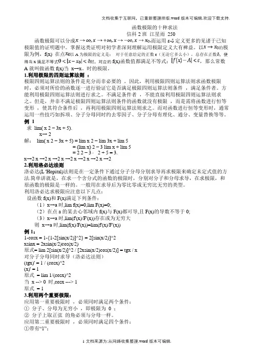
函数极限的十种求法信科2班江星雨250函数极限可以分成而运用ε-δ定义更多的见诸于已知极限值的证明题中。
掌握这类证明对初学者深刻理解运用极限定义大有裨益。
以的极限为例,f(x) 在点以A为极限的定义是:对于任意给定的正数ε(无论它多么小),总存在正数,使得当x满足不等式时,对应的f(x)函数值都满足不等式:,那么常数A就叫做函数f(x)当x→x。
时的极限。
1.利用极限的四则运算法则:极限四则运算法则的条件是充分而非必要的,因此,利用极限四则运算法则求函数极限时,必须对所给的函数逐一进行验证它是否满足极限四则运算法则条件,满足条件者。
方能利用极限四则运算法则进行求之。
不满足条件者,不能直接利用极限四则运算法则求之。
但是,井非不满足极限四则运算法则条件的函数就没有极限,而是需将函数进行恒等变形,使其符合条件后,再利用极限四则运算法则求之。
而对函数进行恒等变形时,通常运用一些技巧如拆项、分子分母同时约去零因子、分子分母有理化、通分、变量替换等等。
例 1求lim( x 2 − 3x + 5).x→ 2解:lim( x 2 − 3x + 5) = lim x 2 − lim 3x + lim 5= (lim x) 2 − 3 lim x + lim 5= 2 2 − 3 ⋅ 2 + 5 = 3.x→2 x →2 x →2 x →2 x →2 x →2 x →22.利用洛必达法则洛必达(L 'Hopital)法则是在一定条件下通过分子分母分别求导再求极限来确定未定式值的方法.简单讲就是,在求一个含分式的函数的极限时,分别对分子和分母求导,在求极限,和原函数的极限是一样的。
一般用在求导后为零比零或无穷比无穷的类型。
利用洛必达求极限应注意以下几点:设函数f(x)和F(x)满足下列条件:(1)x→a时,lim f(x)=0,lim F(x)=0;(2)在点a的某去心邻域内f(x)与F(x)都可导,且F(x)的导数不等于0;(3)x→a时,lim(f'(x)/F'(x))存在或为无穷大则x→a时,lim(f(x)/F(x))=lim(f'(x)/F'(x))例1:1-cosx = 1-{1-2[sin(x/2)]^2} = 2[sin(x/2)]^2xsinx = 2xsin(x/2)cos(x/2)原式= lim 2[sin(x/2)]^2 / [2xsin(x/2)cos(x/2)] = tgx / x对分子分母同时求导(洛必达法则)(tgx)' = 1 / (cosx)^2(x)' = 1原式= lim 1/(cosx)^2当x --> 0 时,cosx ---> 1原式= 13.利用两个重要极限:应用第一重要极限时,必须同时满足两个条件:①分子、分母为无穷小,即极限为0 ;②分子上取正弦的角必须与分母一样。
BULETINUL INSTITUTULUI POLITEHNIC DIN IAŞIPublicat deUniversitatea Tehnică …Gheorghe Asachi” din IaşiTomul LIV (LVIII), Fasc. 3, 2011SecţiaCONSTRUCŢII. ARHITECTURĂPENALTY BASED ALGORITHMS FOR FRICTIONALCONTACT PROBLEMSBYANDREI-IONUŢŞTEFANCU*, SILVIU-CRISTIAN MELENCIUCand MIHAI BUDESCU“Gheorghe Asachi” Technical University of Iaşi,Faculty of Civil Engineering and Building ServicesReceived: June 21, 2011Accepted for publication: August 29, 2011Abstract. The finite element method is a numerical method that can be successfully used to generate solutions for problems belonging to a vast array of engineering fields: stationary, transitory, linear or nonlinear problems. For the linear case, computing the solution to the given problem is a straightforward process, the displacements are obtained in a single step and all the other quantities are evaluated afterwards. When faced with a nonlinear problems, in this case with a contact nonlinearity, one needs to account for the fact that the stiffness matrix of the systems varies with the loading, the force vs. stiffness relation being unknown prior to the beginning of the analysis. Modern software using the finite element method to solve contact problems usually approaches such problems via two basic theories that, although different in their approaches, lead to the desired solutions. One of the theories is known as the penalty function method, and the other as the Lagrange multipliers method. The hereby paper briefly presents the two methods emphasizing the penalty based ones. The paper also underscores the influence of input parameters for the case of the two methods on the results when using the software ANSYS 12.Key words: finite element method; pure penalty methods; Lagrange multipliers method; H-adaptive meshing.*Corresponding author: e-mail: stefancu@ce.tuiasi.ro120Andrei-IonuţŞtefancu, Silviu-Cristian Melenciuc and Mihai Budescu1. IntroductionThe finite element method (FEM) is a numerical method that can be applied to obtain solutions to problems belonging to a variety of engineering disciplines: stationary problems, transitory problems, linear or nonlinear stress/strain problems. Heat transfer, fluid flow, or electromagnetism problems can also be solved using FEM.The first ones to publish articles in this field are Alexander Hrennikoff (1941) and Richard Courant (1943). Although their approaches are different, they have a common feature – discretization of continua into a series of discrete sub-domains called elements. Olgierd Zienkiewicz summarizes the work of his predecessors in what was to be known as FEM (1947). In 1960 Ray Clough is the first one to use the term finite element. Zienkiewicz and Cheung published in 1967 the first book entirely devoted to the finite element method.In this context, in 1971, the first version of the ANSYS software is released. Currently, the ANSYS software package is able to solve static, dynamic, heat transfer, fluid flow, electromagnetics problems, etc. ANSYS is a market leader for more than 20 years (Moavenim, 1999). In the present study version 12.0.1 of the software was used (ANSYS Workbench 2.0, 2009).2. Finite Element Formulations of Contact ProblemsThere are two basic theories that, although different in their approaches, offer the desired solutions to body contact problems: the penalty function method and the Lagrange multipliers method.The main difference between them is the way they include in their formulation the potential energy of contacting surfaces.The penalty function method, due to its economy, has received a wider acceptance. The method is very useful when solving frictional contact problems, while the Lagrange method, based on multipliers, is known for its accuracy.The main drawback of the Lagrange method is that it may lead to ill-converging solutions while the penalty formulation may lead to inaccurate ones.In the following the pure penalty, the augmented Lagrange methods will be presented.2.1. The Penalty MethodThe penalty method involves adding a penalty term to enhance the solving process. In contact problems the penalty term includes the stiffness matrix of the contact surface. The matrix results from the concept that one body imaginary penetrates the another (Wriggers et al., 1990).Bul. Inst. Polit. Ia şi, t. LVII (LXI), f. 3, 2011 121The stiffness matrix of the contact surface is added to the stiffness matrix of the contacting body, so that the incremental equation of the Finite Element becomes[K b + K c ]u = F , (1)where: K b is the stiffness matrix of contacting bodies; K c – stiffness matrix of contact surface; u – displacement; F – force.The magnitude of the contact surface is unknown (Stein & Ramm, 2003), therefore its stiffness matrix, K c , is a nonlinear term. The total load and displacement values are∑Δ=F F tot , (2)∑Δ=u u tot, (3)where: F tot is the force vector; u tot – displacement vector.To derive the stiffness matrix, the contact zone (encompassing the contact surface) is divided into a series of contact elements. The element represents the interaction between the surface node of one body with the respective element face of the other body. Fig. 1 shows a contact element in a two dimensional application. It is composed of a slave node (point S ) and a master line, connecting nodes 1 and 2. S 0 marks the slave node before the application of the load increment, and S marks the node after loading.Fig. 1 – Contact element – penalty method formulation.Given the nature of the numerical simulations presented afterwards only the sliding mode of friction will be presented. In this case, the tangential force acting at the contact surface equals the magnitude of the friction force, hence the first variation of the potential energy of a contact element ist n n d t t n n t t n n c g g k g g g k g f g f δμδδδδ)sgn( +=+=Π, (4)122 Andrei-Ionu ţ Ştefancu, Silviu-Cristian Melenciuc and Mihai Budescuwhere: k n represents penalty terms used to express the relationship between the contact force and the penetrations along the normal direction; k t – penalty terms used to express the relationship between the contact force and the penetrations along the tangential direction; g n – penetration along the normal direction; g t – penetration along the tangential direction;n n n f k g =, (5))()sgn(n n d t t g k g f μ−=. (6)2.2. The Augmented Lagrange Multiplier MethodIn the case of classical Lagrange Multiplier Method the contact forces are expressed by Lagrange multipliers. The augmented Lagrange method involves the regularization of classical Lagrange method by adding a penalty function from the penalty method (Simo & Laursen, 1992). This method, unlike the classical one, can be applied to sticking friction, sliding friction, and to africtionless contactFig. 2 – Contact element – Lagrangian methods.The contact problem involves the minimization of potential П by equating to zero the following expression:kg g g u u T T b 21)(),(+Λ+Π=ΛΠ, (7) where ⎥⎥⎦⎤⎢⎢⎣⎡⎭⎬⎫⎩⎨⎧⎭⎬⎫⎩⎨⎧⎭⎬⎫⎩⎨⎧=Λk t k n t n t n Tλλλλλλ,...,,2211, (8) with:n λ – Lagrange multiplier for the normal direction;t λ– Lagrange multiplier for the tangential direction;Bul. Inst. Polit. Ia şi, t. LVII (LXI), f. 3, 2011 12312k n n n 12k t t t g g g g ,,...,g g g ⎡⎤⎧⎫⎧⎫⎧⎫⎪⎪⎪⎪⎪⎪=⎢⎥⎨⎬⎨⎬⎨⎬⎢⎥⎪⎪⎪⎪⎪⎪⎩⎭⎩⎭⎩⎭⎣⎦. (9)3. Parametric Analysis of Frictional ContactIn order to illustrate the way that the contact algorithms may influence the results a parametric analysis is performed. The purpose of this analysis is to exemplify how various input parameters can alter the results.3.1. Finite Elements Formulations of Contact Problems in ANSYSThe Finite Elements (FE) software ANSYS, for the penalty method, assumes that contact force along the normal direction is written as follows:cont.penetr.cont.F x K Δ=Δ, (10)where: K cont. is the contact stiffness, defined by real constant FKN for the 17x contact elements (in the current analysis the 174 contact element is used); x penetr. – distance between two existing nodes on separate contact bodies; F cont. – contact force. ANSYS automatically chooses the real constant FKN as a scale factor of the stiffness of the underlying elements. This value can be modified by the user (via FKN – a scale factor).Given the fact that the augmented Lagrange method is actually a penalty method with penetration control, the contact force is computed according to eq. (10), the only difference being the contact stiffness formulationpenetr.cont.1x K i i +=+λλ, (11)where λi is a Lagrange multiplier.Although the Lagrange multipliers are condensed out at the element level, one can think regarding this method as the same as a regular penalty one except that the contact stiffness is “updated” per contact element (Imaoka, 2001).Similar to the normal direction, a real constant – FKT models the tangential stiffness of the contact.3.2. Adaptive Solutions in ANSYSIn order to overcome the influence of the meshing upon the final results of the analysis and to improve the accuracy of the solution an adaptive solution will be used.124 Andrei-Ionu ţ Ştefancu, Silviu-Cristian Melenciuc and Mihai BudescuIn ANSYS the desired accuracy of a solution can be achieved by means of adaptive and iterative analysis, whereby h -adaptive methodology is employed.The h -adaptive method begins with an initial FE model that is refined over various iterations by replacing coarse elements with finer ones in selected regions of the model. This is effectively a selective remeshing procedure.The criterion for which elements are selected for adaptive refinement depends on geometry and, for the current analysis, on a 10% allowable difference between the maximum values of the frictional (obtained in two consecutive runs with different meshes).The user-specified accuracy is achieved when convergence is satisfied as follows:)in ...,3,2,1( ,1001R n i E i i i −=<⎟⎠⎞⎜⎝⎛−+φφφ, (11) where:φis the result quantity; E – expected accuracy (10% for this case); R – the region on the geometry that is being subjected to adaptive analysis (entire geometry in this case); i – the iteration number.The results are compared from iteration i to iteration i + 1. Iteration in this context includes a full analysis in which h -adaptive meshing and solving are performed.For this case of adaptive procedures, the ANSYS product identifies the largest elements, which are deleted and replaced with a finer FE representation (ANSYS, 2009).The overall results show a good behavior of the model. Only two iteration are performed in order to satisfy reach the expected accuracy of the solution.Table 1 h-Adaptive Methodology Convergence HistoryIteration Frictional Stress, [MPa]Change, [%] Nodes Elements 1 0.130042,518 352 2 0.12739–2.0571 14,158 8,2343.3. The Model Used in the Parametric AnalysisThe model used, represented in Fig. 3, comprises two solids made up of nonlinear structural steel materials. The larger solid has its lower surface fixed while at the upper end interacts with the smaller solid via a frictional contact (coefficient of friction 0.2). A normal pressure of 0.5 MPa is applied on top of the smaller solid, and displacement is applied on the left hand side face.Bul. Inst. Polit. Iaşi, t. LVII (LXI), f. 3, 2011 125Fig. 3 – The model used in the parametric analysis. A – frictionalcontact; B – applied pressure; C – fixed support; D – applieddisplacement.Input parameters:a) FE formulation (P1); this parameter can take two values: 0 for augmented Lagrange method and 1 for pure penalty method;b) the normal contact stiffness factor FKN (P2) that varies between 0.01 and 1;c) the tangent contact stiffness factor FKT (P3) that varies between 0.01 and 1.Output parameters: a number of output parameters have been monitored, such as: maximum (P5) and minimum (P8) normal elastic strain, maximum (P9) and minimum (P10) shear elastic strain, maximum (P12) and minimum (P13) normal stress, maximum (P14) and minimum (P15) shear stress, maximum (P11) frictional stress, maximum (P6) penetration, analysis run time (P7), maximum stiffness energy (P16).3.4. Results of the Parametric AnalysisThe parametric analysis provides a wide range of information regarding the dependence of the output parameters on the input ones. Based on the relevance of the results only a limited amount of them will be presented.The local sensitivity chart allows one to appreciate the impact of the input parameters on the output ones. This means that the output is computed based on the change of each input independently of the current value of each input parameter. The larger the change of the output, the more significant is the input parameter that was varied (ANSYS, 2009). Since the local sensibilities can only be computed for continuous parameters (P1 is a discrete one) the sensibility chart will be presented for the pure penalty and augmented Lagrange method individually.126Andrei-IonuţŞtefancu, Silviu-Cristian Melenciuc and Mihai BudescuFig. 4 – Local sensibility chart – Lagrangian method.Fig. 5 – Local sensibility chart – pure penalty method.Bul. Inst. Polit. Iaşi, t. LVII (LXI), f. 3, 2011 127It can be seen, from Fig. 5, that the pure penalty method is less sensitiveto contact normal and tangent stiffness than the augmented Lagrange method.The only output parameter influenced by the contact stiffness is the analysisrun-time.In Figs. 4 and 5 only sensitivities of the three parameters (P5, P6, P7)have been presented because the sensitivities of the other are zero or almostzero. Based on this the variation of P5, P6 and P7, with P2 and P3, arepresented in what follows.a bFig. 6 – Variation of P5 with P2 and P3: a – augmented Lagrangemethod; b – pure penalty method.a bFig. 7 – Variation of P6 with P2 and P3: a – augmented Lagrangemethod; b – pure penalty method.As it can be seen from Figs. 6 and 7 there isn’t an exact pattern of thevariation of the maximum normal elastic strain (P5), maximum penetration128Andrei-IonuţŞtefancu, Silviu-Cristian Melenciuc and Mihai Budescu(P6) or analysis run time (P7) with the normal (P2) and tangent (P3) contactstiffness factor.Give the kinematic nature of the problem, and the contact type(frictional) it can be observed from Fig. 8 that the analysis run time (the timeneeded to compute a solution for the given problem) is tangent stiffnessdependent.a bFig. 8 – Variation of P7 with P2 and P3: a – augmented Lagrangemethod; b – pure penalty method.4. ConclusionsGiven the high nonlinear characteristic of the frictional contacts an extraattention is necessary to be paid to contact algorithms and their inputparameters. In such case an h-adaptive solution is recommended to be usedbecause such approach can “fade out” the influence of contact parameters onmost of the output parameters.If working circumstances require fulfilling certain limitations, accuracyconditions may be enforced, thus improving the confidence level of the finalsolution. One must keep in mind though, that an increased number of accuracyconvergence conditions leads to prohibitive analysis run time.REFERENCESClough R.W., The Finite Element Method in Plane Stress Analysis. Proc. 2nd ASCEConf. on Electron. Comp., Pittsburg,Pennsylvania, 1960.Courant R., Variational Methods for the Solution of Problems in Equilibrum and Vibra-tions. Bul. of the Amer. Mathem. Soc., 49,1-23 (1943).Hrennikoff A., Solution of Problems of Elasticity by the Frame-Work Method. ASME,J. of Appl. Mech., 8, 169–175 1(941).Bul. Inst. Polit. Ia şi, t. LVII (LXI), f. 3, 2011 129 Imaoka S., Sheldon’s ANSYS Tips and Tricks: Understanding Lagrange Multipliers .available on-line at /ansys/tips_sheldon/STI07_Lagrange_Mul-tipliers.pdf , 2001.Moavenim A., Finite Element Analysis – Theory and Applicaion with ANSYS . PrenticeHall, Upper Saddle River, New Jersey, 1999.Simo J.C., Laursen T.A., An Augmented Lagrangian Treatment of Contact ProblemsInvolving Friction . Comp. a. Struct., 42, 1, 97-116 (1992).Stein E., Ramm E., Error-Controlled Adaptive Finite Elements in Solid Mechanics . J.Wiley a. Sons, NY, 2003.Wriggers P., Vu Van T., Stein E., Finite Element Formulation of Large DeformationImpact-Contact Problems with Friction . Comp. a. Struct., 37, 3, 319-331 (1990).Zienkiewicz O.C., Cheung Y.K., The Finite Element Method in Continuum andStructural Mechanics . McGraw Hill, NY, 1967.Zienkiewicz O.C., The Stress Distribution in Gravity Dams . J. Inst. Civ. Engng., 27,244-271 (1947). * * * ANSYS Workbench 2.0 Framework Version: 12.0.1. ANSYS Inc., 2009. * * * Design Exploration . ANSYS Inc., 2009. * * * Theory Reference, Analysis Tools, ANSYS Workbench Product Adaptive Solutions . ANSYS Inc., 2009.ALGORITMI BAZA ŢI PE METODA COREC ŢIILOR UTILIZA ŢI ÎNREZOLVAREA PROBLEMELOR DE CONTACT CU FRECARE(Rezumat)Metoda elementului finit este o metod ă numeric ă ce poate fi aplicat ă cu succes pentru a ob ţine solu ţiile problemelor dintr-o multitudine de discipline inginere şti: probleme sta ţionare, probleme tranzitorii, liniare sau neliniare. În cazul liniar g ăsirea solu ţiei unei probleme date este un proces simplu. Deplas ările sunt ob ţinute într-un singur pas de analiz ă, tensiunile şi deforma ţiile fiind evaluate ulterior. În cazul problemelor neliniare – în acest caz neliniaritate de contact – trebuie s ă se ţin ă cont de faptul c ă matricea de rigiditate a sistemului variaz ă func ţie de înc ărcare, rela ţia for ţă vs . rigiditate nefiind cunoscut ă a priori . Programele moderne, ce folosesc metoda elementului finit pentru a rezolva probleme de contact, abordeaz ă de obicei astfel de probleme prin intermediul a dou ă teorii care, de şi diferite în abord ările lor, conduc la solu ţia dorit ă. Una dintre teorii este cunoscut ă sub numele de metoda corec ţiilor, iar cealalt ă ca metoda multiplicatorilor Lagrange. În lucrare se prezint ă pe scurt cele dou ă metode, accentul punându-se pe metodele bazate pe corec ţii. Lucrarea eviden ţiaz ă, de asemenea, influen ţa parametrilor de intrare caracteristici algoritmilor de rezolvare a problemelor de contact asupra rezultatelor atunci când se utilizeaz ă pachetul software ANSYS 12.。
罚函数法及改进算法第3章罚函数法及改进算法引⾔罚函数法是解决约束优化问题的重要⽅法,它的基本思想是⽤⽆约束问题代替约束问题,因⽽⽆约束问题的⽬标函数必须是原来的⽬标函数与约束函数的某种组合,类似线性规划中的M 法求初始可⾏解,在原来的⽬标函数上加上由约束函数组成的⼀个“惩罚项”来迫使迭代点逼近可⾏域,所以称为罚函数法。
这样把约束问题转化成求解⼀系列的⽆约束极⼩点,通过有关的⽆约束问题来研究约束极值问题,从⽽使问题变的简单。
许多⾮线性约束优化⽅法都要⽤罚函数作为评价函数来评价⼀个点的好坏,这在选择新点确定步长等⽅⾯都起着重要的作⽤,不同的罚项对算法影响很⼤,根据罚项的不同可以分为以下⼏类:外罚函数法对于问题min ()f x (3-1).s t ()0i c x = 1,2,,;i m = (3-2)()0i c x ≥ 1,2,,;i m m n =++ (3-3)其中:n f R R →为线性连续函数。
定义外罚函数为:(,)L x σ()()f x P x σ=+()()f x Q x σ=+ (3-4)()Q x =11()min{0,()}m n i i i i m c x c x βα==++∑∑ (3-5) 通常取==2αβ,这样定义的外罚函数法,当x 为可⾏点是,()0Q x =;当x 不是可⾏点时,()0Q x >。
⽽且x 离可⾏域越远()Q x 的值越⼤,它优点是允许从可⾏域的外部逐步逼近最优点,但其明显的缺点是它需要求解⼀系列⽆约束极⼩化问题,计算⼯作量很⼤,且由于其收敛速度仅是线性的,往往需要较长的时间才能找到问题的近似解,再考虑到实际中所使⽤的终⽌准则,若实现不当,则算法很难找到约束问题的⼀个较好可⾏解,从⽽不适⽤于那些要求严格可⾏性的问题。
内罚函数法它是针对不等式约束(3-1)(3-3)提出的,基本思想是在约束区域的边界筑起⼀道“墙”来,当迭代点靠近边界时,函数值陡然增⼤,于是最优点被挡在可⾏域内部,这样产⽣的点列k x 每个点都是可⾏点。
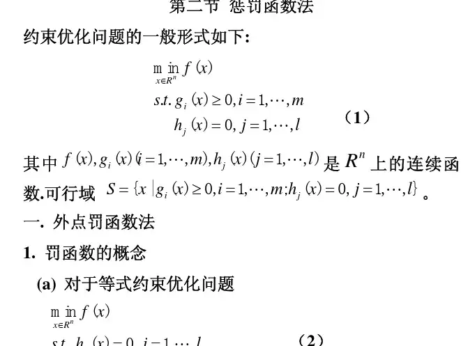
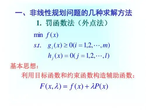
罚函数法罚函数法是能够处理一般的约束优化问题:min ()()0,1,2,()0,1,2,,i if x h x i kg x j m ⎧⎪==⎨⎪≥=⎩ 的一类方法。
其基本思想是将约束优化问题卑微无约束问题来求解。
罚函数是由目标函数和约束函数的某种组合得到的函数,对于等式约束的优化问题min ()()0,1,2,i f x h x i k⎧⎨==⎩ ,可以定义如下的罚函数: 21()()()ki i F x f x c h x ==+∑将约束优化问题转化为无约束优化问题;对于不等式约束的优化问题min ()()0,1,2,,i f x g x j m⎧⎨≥=⎩ 可以定义如下的罚函数:11()()()mj j F x f x C g x ==+∑对于同时存在等式约束和不等式约束的优化问题,可以去上面两个罚函数的组合。
当然罚函数还有其他的取法,但是构造罚函数的思想都是一样的,即使得在可行点罚函数等于原来的目标函数值,在不可行点罚函数等于一个很大的数。
外点罚函数法 1.算法原理外点罚函数法是通过一系列罚因子{}i c ,求罚函数的极小值来逼近原约束问题的最有点。
之所以称为外点罚函数法,是因为它是从可行域外部向约束边界逐步靠拢的。
2,。
算法步骤用外点罚函数法求解线性约束问题min ()f x Ax b ⎧⎨=⎩的算法过程如下:1,给定初始点(0)x ,罚参数列{}i c 及精度0ε>,置1k =; 2,构造罚函数2()()F x f x c Ax b =+-;3,用某种无约束非线性规划,以(1)k x -为初始点求解min ()F x ;4,设最优解为()k x ,若()k x 满足某种终止条件,则停止迭代输出()k x ,否则令1k k =+,转2;罚参数列{}i c 的选法:通常先选定一个初始常数1c 和一个比例系数2ρ≥,则其余的可表示为11i i c c ρ-=。
终止条件可采用()S x ε≤,其中2()S x c Ax b =-。
浓度问题一个好玩的故事——熊喝豆浆黑熊领着三个弟弟在森林里游玩了半天,感到又渴又累,正好路过了狐狸开的豆浆店。
只见店门口张贴着广告:“既甜又浓的豆浆每杯0.3元。
”黑熊便招呼弟弟们歇脚,一起来喝豆浆。
黑熊从狐狸手中接过一杯豆浆,给最小的弟弟喝掉61,加满水后给老三喝掉了31,再加满水后,又给老二喝了一半,最后自己把剩下的一半喝完。
狐狸开始收钱了,他要求黑熊最小的弟弟付出0.3×61=0.05(元);老三0.3×31=0.1(元);老二与黑熊付的一样多,0.3×21=0.15(元)。
兄弟一共付了0.45元。
兄弟们很惊讶,不是说,一杯豆浆0.3元,为什么多付0.45-0.3=0.15元?肯定是黑熊再敲诈我们。
不服气的黑熊嚷起来:“多收我们坚决不干。
”“不给,休想离开。
”现在,说说为什么会这样呢?专题简析:溶质:在溶剂中的物质。
溶剂:溶解溶质的液体或气体。
溶液:包含溶质溶剂的混合物。
在小升初应用题中有一类叫溶液配比问题,即浓度问题。
我们知道,将糖溶于水就得到了糖水,其中糖叫溶质,水叫溶剂,糖水叫溶液。
如果水的量不变,那么糖加得越多,糖水就越甜,也就是说糖水甜的程度是由糖(溶质)与糖水(溶液=糖+水)二者质量的比值决定的。
这个比值就叫糖水的含糖量或糖含量。
类似地,酒精溶于水中,纯酒精与酒精溶液二者质量的比值叫酒精含量。
因而浓度就是溶质质量与溶液质量的比值,通常用百分数表示,即,浓度=溶质质量溶液质量×100%=溶质质量溶质质量+溶剂质量×100%相关演化公式溶质的重量+溶剂的重量=溶液的重量溶质的重量÷溶液的重量×100%=浓度溶液的重量×浓度=溶质的重量溶质的重量÷浓度=溶液的重量解答浓度问题,首先要弄清什么是浓度。
在解答浓度问题时,根据题意列方程解答比较容易,在列方程时,要注意寻找题目中数量问题的相等关系。
浓度问题变化多,有些题目难度较大,计算也较复杂。
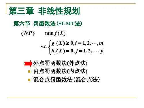
第十章 罚函数法与广义乘子法本章主要内容:外罚函数法 内罚函数法 广义乘子法教学目的及要求:了解外罚函数法、内罚函数法、广义乘子法。
教学重点:外罚函数法. 教学难点:广义乘子法. 教学方法:启发式.教学手段:多媒体演示、演讲与板书相结合. 教学时间:3学时. 教学内容:§10.1 外罚函数法考虑约束非线性最优化问题min ();()0,1,2,,,()0,1,2,,,i j f x g x i m h x j l ⎧⎪≥=⎨⎪==⎩s.t. (10.1.1)其中(),()1,2,,()1,2,,i j f x g x i m h x j l ==()和()都是定义在n R 上的实值连续函数.记问题(10.1.1)的可行域为S .对于等式约束问题min ();()0,1,2,,,j f x h x j l ⎧⎨==⎩s.t. (10.1.2)定义罚函数211(,)()()lj j F x f x h x σσ==+∑,其中参数σ是很大的正常数.这样,可将问题(10.1.2)转化为无约束问题 1min (,)nx RF x σ∈. (10.1.3) 对于不等式约束问题min ();()0,1,2,,,i f x g x i m ⎧⎨≥=⎩s.t. (10.1.4)定义罚函数221(,)()[max{0,()}]mi i F x f x g x σσ==+-∑,其中σ是很大的正数.这样,可将问题(10.1.4)转化为无约束问题2min (,)nx RF x σ∈. (10.1.5) 对于一般的约束最优化问题(10.1.1),定义罚函数 (,)()()F x f x P x σσ=+, 其中σ是很大的正数,()P x 具有下列形式:11()[()][()]mli j i j P x g x h x ϕφ===+∑∑.ϕ和φ是满足下列条件的实值连续函数:()0,0()0,0y y y y ϕϕ=≥⎧⎨><⎩当时,当时, ()0,0()0,0y y y y φφ==⎧⎨>≠⎩当时,当时.函数ϕ和φ的典型取法为()[max{0,}]y y αϕ=-, ()||y y βφ=,其中1α≥和1β≥是给定的常数,通常取作1或2.这样,可将约束问题(10.1.1)转化为无约束问题min (,)()()nx RF x f x P x σσ∈=+, (10.1.6) 其中σ是很大的正数,()P x 是连续函数.算法10-1(外罚函数法)Step1 选取初始数据.给定初始点0x ,初始罚因子10σ>,放大系数1α>,允许误差0ε>,令1k =.Step2 求解无约束问题.以1k x -为初始点,求解无约束问题min (,)()()nx RF x f x P x σσ∈=+, (10.1.11) 设其最优解为k x .Step3 检查是否满足终止准则.若()k k P x σε<,则迭代终止,k x 为约束问题(10.1.1)的近似最优解;否则,令1,:1k k k k σασ+==+,返回Step2.例1 用外罚函数法在平面23x y +=上求一点(,)P x y ,使得P 到定点(3,2)A 的距离近似最短,取310.5,2,10σαε-===.解 令22(,)(3)(2)f x y x y =-+-,问题可归为求解如下最优化问题22min (,)(3)(2);(,)230.f x y x y h x y x y ⎧=-+-⎨=+-=⎩s.t.引入罚函数 222(,,)(3)(2)(23)k k F x y x y x y σσ=-+-++-. 则原约束最优化问题相应的一系列无约束最优化问题为:min (,,)k F x y σ,其中110.5,2,1,2,k k k σσσ+===.解上述无约束问题,得31122(,),1515TT k k k k k k x y σσσσ⎛⎫++= ⎪++⎝⎭,同时216(,)(15)kk k k k P x y σσσ=+. 依次对1,2,k =用上述公式计算(,)T k k x y 和(,)k k k P x y σ,结果如下表所示.由迭代终止条件3216(,)10(15)k k k k k P x y σσσ-=<+可得原约束问题的近似最优解(保留4位有效数字)1212(,)(2.2002,0.4003)T T x y =.§10.2 内罚函数法对于不等式约束问题(10.1.4),其可行域S 的内部int {|,()0,1,2,,}n i S x x R g x i m =∈>=.为了保持迭代点始终含于int S ,我们引入另一种罚函数(,)()()G x r f x rB x =+,其中r 是很小的正数,()B x 是int S 上的非负实值连续函数,当点x 趋向可行域S 的边界时,()B x →∞.显然,罚函数(,)G x r 的作用是对企图脱离可行域的点给予惩罚,相当于在可行域的边界设置了障碍,不让迭代点穿越到可行域之外,因此也称为障碍函数. (,)G x r 的两种常用的形式为11(,)()()mi i G x r f x r g x ==+∑, 及1(,)()ln ()mi i G x r f x r g x ==-∑分别称为倒数障碍函数和对数障碍函数.算法10-2(内罚函数法或SUMT 内点法)Step1 选取初始数据.给定初始内点0int x S ∈,初始参数10r >,缩小系数(0,1)β∈,允许误差0ε>,令1k =.Step2 求解无约束问题.以1k x -为初始点,求解无约束问题min (,)()();int ,k k G x r f x r B x x S =+⎧⎨∈⎩s.t. (10.2.2)设其最优解为k x .Step3 检查是否满足终止准则.若()k k r B x ε<,则迭代终止,k x 为约束问题(10.1.4)的近似最优解;否则,令1,:1k k r r k k β+==+,返回Step2.算法10-3(求内罚函数法中初始内点的算法)Step1 选取初始数据.给定初始点0x ,初始参数10r >,缩小系数(0,1)β∈,令1k =.Step2 确定指标集.令{|()0,1,2,,}k i k I i g x i m =≤=,{|()0,1,2,,}k i k J i g x i m =>=.Step3 检验是否满足终止准则.若k I =∅,则int k x S ∈,迭代终止;否则,转Step4.Step4 求解无约束问题.以k x 为初始点,求无约束问题1min ()kk x S H x +∈的最优解1k x +,其中111()()()kkk i k i I i J i H x g x r g x ++∈∈=-+∑∑, {|()0,}k i k S x g x i J =>∈.令21,:1k k r r k k β++==+,返回Step2.§10.3 广义乘子法考虑只带等式约束的最优化问题(10.1.2).不难知道,问题(10.1.2)等价于问题21min ()();2()0,1,2,,,l j j j f x h x h x j l σ=⎧⎡⎤+⎪⎢⎥⎨⎣⎦⎪==⎩∑s.t. (10.3.1)其中0σ>.该问题的Lagrange 函数211(,,)()()()2l ljj jj j L x v f x h x v h x σσ===+-∑∑, 由于(,,)L x v σ中既有罚项21()2ljj h x σ=∑,又有乘子项1()lj jj v h x =-∑,故称为乘子罚函数.与外罚函数类似,若设{}k σ为严格单调递增且趋于无穷大的正数列,则我们可以把求解等式约束问题(10.1.2)转化为求解一系列的无约束问题2()11min (,,)()()()2nl lk kk k j jj x Rj j L x v f x h x vh x σσ∈===+-∑∑, (10.3.2)其中()()()12(,,,)k k k T k l v v v v =是第k 次迭代中采用的Lagrange 乘子,并且有定理10.3.1 设k x 是无约束问题(10.3.2)的最优解,则k x 也是问题min ();()(),1,2,,j j k f x h x h x j l⎧⎨==⎩s.t. (10.3.3)的最优解.记12()((),(),,())T l h x h x h x h x =.算法10-4(等式约束下的广义乘子法)Step1 选取初始数据.给定初始点0x ,初始乘子1v ,初始罚因子10σ>,放大系数1α>,允许误差0ε>,参数(0,1)γ∈,令1k =.Step2 求解无约束问题.以1k x -为初始点,求解无约束问题(10.3.2),设其最优解为k x .Step3 检查是否满足终止准则.若()k h x ε<,则迭代终止,k x 为等式约束问题(10.1.2)的近似最优解;否则,转Step4.Step4 判断收敛快慢.若1()()k k h x h x γ-≥,则令1k k σασ+=,转Step5;否则,令1:k k σσ+=,转Step5.Step5 进行乘子迭代.令(1)()(),1,2,,,:1k k j j k j k v v h x j l k k σ+=-==+,返回Step2.。