利用cvMinAreaRect2求取轮廓最小外接矩形

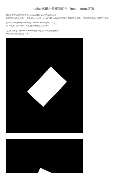
matlab求最⼩外接斜矩形minboundrect⽅法最近在做课程⼤作业时看到opencv函数cv2.minAreaRect()，但是想⽤matlab实现，于是查到了John D’Errico写的matlab实现求最⼩外接斜矩形函数。

（代码贴在最后，仅供学习使⽤）[rectx,recty,area,perimeter] = minboundrect(c,r,‘a’)其中a表⽰以⾯积最⼩、如果是p的话则是以边长最⼩这⾥有个问题，⽤minboundrect函数求得的四个点顺序是什么？于是做了两张图验证了⼀下放上结果：可以得到minboundrect函数得到的结果(rectx,recty)是从最上边的点开始，按照顺时针⽅向索引。

minboundrect代码function[rectx,recty,area,perimeter]=minboundrect(x,y,metric)% minboundrect: Compute the minimal bounding rectangle of points in the plane% usage:[rectx,recty,area,perimeter]=minboundrect(x,y,metric)%% arguments:(input)% x,y - vectors of points, describing points in the plane as%(x,y) pairs. x and y must be the same lengths.%% metric -(OPTIONAL)- single letter character flag which% denotes the use of minimal area or perimeter as the% metric to be minimized. metric may be either 'a' or 'p',% capitalization is ignored. Any other contraction of'area'% or 'perimeter' is also accepted.%%DEFAULT:'a'('area')%% arguments:(output)% rectx,recty -5x1 vectors of points that define the minimal% bounding rectangle.%% area -(scalar) area of the minimal rect itself.%% perimeter -(scalar) perimeter of the minimal rect as found%%% Note: For those individuals who would prefer the rect with minimum% perimeter or area, careful testing convinces me that the minimum area% rect was generally also the minimum perimeter rect on most problems%(with one class of exceptions). This same testing appeared to verify my% assumption that the minimum area rect must always contain at least% one edge of the convex hull. The exception I refer to above is for% problems when the convex hull is composed of only a few points,% most likely exactly 3. Here one may see differences between the% most likely exactly 3. Here one may see differences between the % two metrics. My thanks to Roger Stafford for pointing out this%class of counter-examples.%% Thanks are also due to Roger for pointing out a proof that the% bounding rect must always contain an edge of the convex hull,in % both the minimal perimeter and area cases.%%% Example usage:% x =rand(50000,1);% y =rand(50000,1);% tic,[rx,ry,area]=minboundrect(x,y);toc%% Elapsed time is 0.105754 seconds.%%[rx,ry]% ans =%0.99994-4.2515e-06%0.999980.99999% 2.6441e-051%-5.1673e-06 2.7356e-05%0.99994-4.2515e-06%% area% area =%0.99994%%% See also: minboundcircle, minboundtri, minboundsphere%%% Author: John D'Errico%E-mail: woodchips@% Release:3.0% Release date:3/7/07%default for metricif(nargin<3)||isempty(metric)metric ='a';elseif ~ischar(metric)error 'metric must be a character flag if it is supplied.'else% check for'a' or 'p'metric =lower(metric(:)');ind =strmatch(metric,{'area','perimeter'});if isempty(ind)error 'metric does not match either ''area'' or ''perimeter'''end% just keep the first letter.metric =metric(1);end% preprocess datax=x(:);y=y(:);% not many error checks to worry aboutn =length(x);if n~=length(y)error 'x and y must be the same sizes'end% start out with the convex hull of the points to% reduce the problem dramatically. Note that any% reduce the problem dramatically. Note that any% points in the interior of the convex hull are% never needed, so we drop them.if n>3edges =convhull(x,y);%edges =convhull(x,y,{'Qt'});%'Pp' will silence the warnings% exclude those points inside the hull as not relevant% also sorts the points into their convex hull as a% closed polygonx =x(edges);y =y(edges);% probably fewer points now, unless the points are fully convex nedges =length(x)-1;elseif n>1% n must be 2 or 3nedges = n;x(end+1)=x(1);y(end+1)=y(1);else% n must be 0 or 1nedges = n;end% now we must find the bounding rectangle of those% that remain.% special case small numbers of points. If we trip any%of these cases, then we are done, so return.switch nedgescase0% empty begets emptyrectx =[];recty =[];area =[];perimeter =[];returncase1%with one point, the rect is simple.rectx =repmat(x,1,5);recty =repmat(y,1,5);area =0;perimeter =0;returncase2% only two points. also simple.rectx =x([12211]);recty =y([12211]);area =0;perimeter =2*sqrt(diff(x).^2+diff(y).^2);returnend%3 or more points.% will need a 2x2 rotation matrix through an angle thetaRmat = @(theta)[cos(theta)sin(theta);-sin(theta)cos(theta)];%get the angle of each edge of the hull polygon.ind =1:(length(x)-1);edgeangles =atan2(y(ind+1)-y(ind),x(ind+1)-x(ind));% move the angle into the first quadrant.edgeangles =unique(mod(edgeangles,pi/2));% now just check each edge of the hull% now just check each edge of the hullnang =length(edgeangles);area = inf;perimeter = inf;met = inf;xy =[x,y];for i =1:nang% rotate the data through -thetarot =Rmat(-edgeangles(i));xyr = xy*rot;xymin =min(xyr,[],1);xymax =max(xyr,[],1);% The area is simple,as is the perimeterA_i =prod(xymax - xymin);P_i =2*sum(xymax-xymin);if metric=='a'M_i = A_i;elseM_i = P_i;end%new metric value for the current interval. Is it better?if M_i<met% keep this onemet = M_i;area = A_i;perimeter = P_i;rect =[xymin;[xymax(1),xymin(2)];xymax;[xymin(1),xymax(2)];xymin]; rect = rect*rot';rectx =rect(:,1);recty =rect(:,2);endend%get the final rect% all doneend % mainline end代码仅供学习。

10、最小外接矩形及长宽的求法liuqingjie2@#include "cv.h"#include "highgui.h"#include <stdio.h>#include <math.h>#include "otsu.h"int main(int argc,char** argv){IplImage *src,*gray,*bw,*dst;CvMemStorage* storage=cvCreateMemStorage(0);CvSeq* contour=0;char* filename=argc==2?argv[1]:"5.jpg";if(!filename)printf("can't open the file:%d\n",filename);src=cvLoadImage(filename,1);cvNamedWindow("image",1);cvShowImage("image",src);gray=cvCreateImage(cvSize(src->width,src->height),src->depth,1);cvCvtColor(src,gray,CV_BGR2GRAY);hei=gray->height;//注意此处是gray，otsu中要用到hei,wid,已在otsu.h中全局定义；wid=gray->width;printf("图像的高为：%d,宽为：%d\n\n",hei,wid);cvNamedWindow("image2",1);cvShowImage("image2",gray);bw=cvCreateImage(cvGetSize(src),IPL_DEPTH_8U,1);otsu(gray,bw);cvNamedWindow("image4",1);cvShowImage("image4",bw);// wb=cvCloneImage(bw);// cvNot(bw,wb); 只有当目标区域为黑色背景时候，才对其取反。

最小外接矩形原理最小外接矩形原理是一种经典的计算几何方法，它用于解决问题如何用最小的矩形来包含给定的点集。

这个方法在图形识别、图像处理、计算机视觉、机器人控制等领域得到广泛应用。

1. 整体思路最小外接矩形算法的核心思想是寻找包围点集的最小矩形，这个矩形的特点是其边缘经过点集上的某些点。

仿佛在给一个矩形铁丝网，然后用手将它塚在点集上使得这个矩形的边正好经过点集上某些点，这样得到的矩形就是最小外接矩形（Minimum Bounding Rectangle，MBR）。

2. 算法分类一般而言，最小外接矩形算法有两种种类：顺时针旋转和平面扫描。

顺时针旋转法：顺时针旋转法的基本思路是将点集沿逆时针方向旋转，然后找到对应点集的最小外接矩形。

这个算法可以使用旋转角度的技术来实现，并在选出最小包围矩形时实时更新候选矩形。

平面扫描法：平面扫描算法通常基于一个简单和直观的想法，即按特定方向将点集排序，并查找距离相同的两个点，在这样的基础上，可以根据其距离和方向构建最小包围矩形。

3. 算法实现无论采用什么样的算法，最小外接矩形的实现主要分为以下几个步骤：· 先找到点集中的最大和最小x、y坐标，并计算出矩形的初始宽度和高度。

· 将初始矩形的中心放在点集的中心，并旋转最小旋转角度，更新最优矩形（距离=宽度×高度）。

· 从该点向其他点扫描，并计算得到其他可能的包围矩形，最终找到最小的包围矩形。

相比平面扫描法，旋转法相对简单明了，我们这里就以旋转法为例进行实践。

C++代码实现如下：```c++ #include<iostream> #include<cstdio>#include<cmath> #include<algorithm> using namespace std; #define maxn 100005 const double eps=1e-10; // 浮点数的eps struct complex { double x,y; complex(double x=0,double y=0):x(x),y(y) {} };inline complex operator +(complex a,complexb){return complex(a.x+b.x,a.y+b.y);} inline complexoperator -(complex a,complex b){return complex(a.x-b.x,a.y-b.y);} inline complex operator *(complexa,complex b){return complex(a.x*b.x-a.y*b.y,a.x*b.y+a.y*b.x);}int n,top; double d[maxn],ans_w,ans_h; complexp[maxn],st[maxn],h[maxn],w,var;inline double dist(complex a,complex b) {returnsqrt((b.x-a.x)*(b.x-a.x)+(b.y-a.y)*(b.y-a.y));} //计算距离inline bool cmp(const complex &a,const complex&b) { return (a.x==b.x)?(a.y<b.y):(a.x<b.x); } inline double angle(complex a) {returnatan2(a.y,a.x);} inline double ang(complexa,complex b,complex c) {return fabs(angle(a-b)-angle(c-b));}inline void init() { top=1;sort(p+1,p+1+n,cmp); for(int i=1;i<=n;++i){ while(top>1 && (h[top]-h[top-1])*(p[i]-h[top-1])<=0) --top;h[++top]=p[i]; } w=h[top]-h[1]; for(inti=2;i<top;++i)if(ang(h[1],h[i],h[top])<ang(h[1],w,h[top]))w=h[i]-h[1]; for(int i=1;i<=top;++i)d[i]=dist(h[i],h[i%top+1]); }inline void solve() { int j=2;var.x=ans_w; var.y=ans_h; for(inti=1;i<=top;++i){ while((w*(h[i]+st[j])-w*st[j-1]).y >=0) j=j+1>top?1:j+1; // 更新答案double new_w=dist(h[i],st[j]), new_h=fabs((w*(h[i]-st[j])).y); if(new_w*var.y-var.x*new_h<ans_w*ans_h*eps){ ans_w=new_w; ans_h=new_h;var.x=ans_w;var.y=ans_h; } } }int main() { int T; scanf("%d",&T);while(T--) { scanf("%d",&n);for(int i=1;i<=n;++i)scanf("%lf%lf",&p[i].x,&p[i].y); if(n==1){ printf("0.00\n"); continue; } init();ans_w=hypot(w.x,w.y);ans_h=0; // 初始答案solve(); swap(ans_w,ans_h);printf("%.2lf\n",ans_w*ans_h); if(T)printf("\n"); } return 0; } ```4. 总结最小外接矩形算法是一种实用的算法，在很多计算机应用中有着广泛的应用。

最小外接矩形主轴法一、最小外接矩形与主轴法的定义最小外接矩形（Minimum Bounding Rectangle，MBR）是一种用于描述二维空间中点集或几何形状边界的最小矩形的方法。

主轴法（Major Axis Theorem）是一种基于几何原理，通过找到最小外接矩形的中心点和主轴来确定矩形的方法。

二、主轴法原理及其算法实现主轴法的基本原理是找到一个方向，使得在该方向上最小外接矩形的边界点到中心的距离最小。

这个方向就是最小外接矩形的主轴方向。

在二维空间中，最小外接矩形有水平和垂直两个主轴方向。

算法实现上，首先需要计算所有点的质心，然后找到围绕质心旋转的点集分布的旋转主轴。

通过旋转主轴和质心可以确定最小外接矩形的两个主轴方向。

最后，根据主轴方向和质心坐标可以确定最小外接矩形的四个角点坐标。

三、主轴法在最小外接矩形计算中的应用主轴法在最小外接矩形计算中有广泛的应用。

例如，在地图分析、数据可视化、计算机图形学、模式识别等领域中，经常需要计算一组点或形状的最小外接矩形。

通过使用主轴法，可以快速准确地找到这些矩形，进而进行进一步的分析和处理。

四、最小外接矩形主轴法的优缺点优点：1.算法简单易实现，计算速度快。

2.可以快速准确地找到最小外接矩形。

3.可以处理任意形状和方向的点集或几何形状。

缺点：1.对于一些特殊形状的点集或几何形状，可能会出现主轴方向的判断误差，影响计算精度。

2.对于一些边界模糊或不规则的点集或几何形状，最小外接矩形的计算结果可能会不准确。

3.在高维空间中，最小外接矩形的计算变得更加复杂，需要更高级的算法和技术。

五、主轴法在计算机图形学中的其他应用除了最小外接矩形计算，主轴法在计算机图形学中还有其他应用。

例如，在碰撞检测中，可以使用主轴法快速判断两个物体是否相交；在动画制作中，可以使用主轴法确定物体旋转的中心点和旋转方向；在几何变换中，可以使用主轴法确定旋转、平移等变换操作的中心点和方向。

halcon-smallest_rectangle2返回最⼩外接任意⾓度矩形数据最⼩外接矩形：最⼩外接矩形长宽的⼀半称为长宽半轴，长轴⽅向称为区域的⽅向存在任意⾓度的称为rect2，⽔平竖直的矩形称为rect1在HDevelop中read_image (Image, 'D:/bb/tu/5.jpg')rgb1_to_gray(Image,Image1)threshold (Image1, Region,[75] , [90])smallest_rectangle2 (Region, Row, Column, Phi, Length1, Length2)*返回最⼩外接任意⾓度矩形数据*参数1：输⼊区域*参数2：最⼩外接矩形的中⼼点的⾏坐标-y坐标*参数3：最⼩外接矩形的中⼼点的列坐标-x坐标*参数4：最⼩外接矩形的长边与图像坐标系x轴的夹⾓,，范围为-1.5707963265到+1.5707963265弧度（-90°到+90°）* x轴算起逆时针时⾓度为正，顺时针是⾓度为负*参数5：最⼩外接矩形的短边（宽度 width）*参数6：最⼩外接矩形的长边（长度 height）get_image_size (Image1, Width, Height)dev_open_window(10,10,Width, Height,'black',WindowHandle)dev_display(Region)dev_open_window(10,10,Width, Height,'black',WindowHandle1)gen_rectangle2(Rectangle,Row,Column,Phi,Length1,Length2)*⽣成任意⾓度矩形区域*参数1：Rectangle输出任意⾓度矩形区域*参数2：Row 矩形中⼼点⾏坐标*参数3：Column矩形中⼼点列坐标*参数4：Phi⾓度*参数5：Length1矩形宽度的⼀半*参数6：Length2矩形长度的⼀半dev_display(Rectangle)在QtCreator中HObject ho_Image, ho_Image1, ho_Region, ho_Rectangle;HTuple hv_Row, hv_Column, hv_Phi, hv_Length1;HTuple hv_Length2, hv_Width, hv_Height, hv_WindowHandle;HTuple hv_WindowHandle1;ReadImage(&ho_Image, "D:/bb/tu/5.jpg");Rgb1ToGray(ho_Image, &ho_Image1);Threshold(ho_Image1, &ho_Region, 75, 90);SmallestRectangle2(ho_Region, &hv_Row, &hv_Column, &hv_Phi, &hv_Length1, &hv_Length2);//返回最⼩外接任意⾓度矩形数据//参数1：输⼊区域//参数2：最⼩外接矩形的中⼼点的⾏坐标-y坐标//参数3：最⼩外接矩形的中⼼点的列坐标-x坐标//参数4：最⼩外接矩形的长边与图像坐标系x轴的夹⾓,，范围为-1.5707963265到+1.5707963265弧度（-90°到+90°）// x轴算起逆时针时⾓度为正，顺时针是⾓度为负//参数5：最⼩外接矩形的短边（宽度 width）//参数6：最⼩外接矩形的长边（长度 height）GetImageSize(ho_Image1, &hv_Width, &hv_Height);SetWindowAttr("background_color","black");OpenWindow(10,10,hv_Width,hv_Height,0,"visible","",&hv_WindowHandle);HDevWindowStack::Push(hv_WindowHandle);if (HDevWindowStack::IsOpen())DispObj(ho_Region, HDevWindowStack::GetActive());SetWindowAttr("background_color","black");OpenWindow(10,10,hv_Width,hv_Height,0,"visible","",&hv_WindowHandle1);HDevWindowStack::Push(hv_WindowHandle1);GenRectangle2(&ho_Rectangle, hv_Row, hv_Column, hv_Phi, hv_Length1, hv_Length2);//⽣成任意⾓度矩形区域//参数1：Rectangle输出任意⾓度矩形区域//参数2：Row 矩形中⼼点⾏坐标//参数3：Column矩形中⼼点列坐标//参数4：Phi⾓度//参数5：Length1矩形宽度的⼀半//参数6：Length2矩形长度的⼀半if (HDevWindowStack::IsOpen())DispObj(ho_Rectangle, HDevWindowStack::GetActive());。

在OpenCV中，使用函数minAreaRect来计算给定点集的最小外接矩形在OpenCV中，可以使用函数minAreaRect来计算给定点集的最小外接矩形。

最小外接矩形是将所有的点包含在内的最小面积的矩形。

以下是使用OpenCV进行最小外接矩形计算的示例代码：import cv2import numpy as np# 创建一个点集points = np.array([[50, 50], [150, 50], [150, 150], [50, 150]], dtype=np.int32)# 计算最小外接矩形rect = cv2.minAreaRect(points)# 提取最小外接矩形的中心点、宽高和旋转角度(center, size, angle) = rect# 将浮点型数据转为整数center = (int(center[0]), int(center[1]))size = (int(size[0]), int(size[1]))# 绘制最小外接矩形，并显示image = np.zeros((200, 200, 3), dtype=np.uint8)cv2.drawContours(image, [points], -1, (0, 255, 0), 2)box = cv2.boxPoints(rect).astype(int)cv2.drawContours(image, [box], -1, (0, 0, 255), 2)cv2.imshow('Minimum Enclosing Rectangle', image)cv2.waitKey(0)cv2.destroyAllWindows()在上述代码中，我们首先创建了一个点集points，它包含了四个点的坐标。

然后使用minAreaRect函数计算最小外接矩形的相关信息，包括中心点坐标、宽高和旋转角度。

接着，我们使用drawContours函数绘制了原始点集和最小外接矩形，并将结果显示出来。

minarearect参数Minarearect参数是OpenCV中的一个函数，用于在图像中检测并绘制出最小面积矩形。

这个函数在计算机视觉和图像处理领域中具有广泛的应用。

本文将介绍minarearect参数的使用方法和其在图像处理中的应用。

我们来了解一下minarearect参数的基本用法。

在OpenCV中，minarearect参数是用于在二值图像中检测最小面积矩形的函数。

它可以找到图像中所有轮廓的外接最小面积矩形，并将其绘制出来。

使用minarearect参数的步骤如下：1. 将图像转换为二值图像。

可以使用阈值分割或其他图像处理方法将图像转换为二值图像。

2. 使用findContours函数找到图像中的所有轮廓。

这些轮廓是图像中的连续像素点集合。

3. 对每个轮廓，使用minarearect参数计算其外接最小面积矩形。

4. 将计算得到的最小面积矩形绘制到原始图像中。

通过使用minarearect参数，我们可以在图像中定位并绘制出最小面积矩形。

这在很多图像处理任务中都非常有用，例如目标检测、图像分割、形状识别等。

在目标检测任务中，minarearect参数可以帮助我们找到图像中的目标物体，并计算出其位置和方向。

通过计算最小面积矩形的中心点坐标和旋转角度，我们可以确定目标物体在图像中的位置和朝向。

在图像分割任务中，minarearect参数可以用于分割不规则形状的物体。

通过计算最小面积矩形，我们可以将图像中的物体区域与背景区域分离开来，从而实现图像分割的目的。

在形状识别任务中，minarearect参数可以用于识别图像中的形状。

通过计算最小面积矩形的长宽比例和角度，我们可以判断出图像中的形状类型，例如矩形、正方形、长方形等。

除了上述应用之外，minarearect参数还可以用于图像匹配、图像配准、图像纠偏等任务。

它在计算机视觉和图像处理领域中具有广泛的应用前景。

minarearect参数是OpenCV中一个非常有用的函数，可以帮助我们在图像中检测并绘制出最小面积矩形。

pythonopencvminAreaRect⽣成最⼩外接矩形的⽅法使⽤python opencv返回点集cnt的最⼩外接矩形，所⽤函数为 cv2.minAreaRect(cnt) ，cnt是点集数组或向量（⾥⾯存放的是点的坐标），并且这个点集不定个数。

举例说明：画⼀个任意四边形（任意多边形都可以）的最⼩外接矩形，那么点集 cnt 存放的就是该四边形的4个顶点坐标（点集⾥⾯有4个点）cnt = np.array([[x1,y1],[x2,y2],[x3,y3],[x4,y4]]) # 必须是array数组的形式rect = cv2.minAreaRect(cnt) # 得到最⼩外接矩形的（中⼼(x,y), (宽,⾼), 旋转⾓度）box = cv2.cv.BoxPoints(rect) # cv2.boxPoints(rect) for OpenCV 3.x 获取最⼩外接矩形的4个顶点坐标box = np.int0(box)函数 cv2.minAreaRect() 返回⼀个Box2D结构rect：（最⼩外接矩形的中⼼（x，y），（宽度，⾼度），旋转⾓度），但是要绘制这个矩形，我们需要矩形的4个顶点坐标box, 通过函数 cv2.cv.BoxPoints() 获得，返回形式[ [x0,y0], [x1,y1], [x2,y2], [x3,y3] ]。

得到的最⼩外接矩形的4个顶点顺序、中⼼坐标、宽度、⾼度、旋转⾓度（是度数形式，不是弧度数）的对应关系如下：注意：旋转⾓度θ是⽔平轴（x轴）逆时针旋转，与碰到的矩形的第⼀条边的夹⾓。

并且这个边的边长是width，另⼀条边边长是height。

也就是说，在这⾥，width与height不是按照长短来定义的。

在opencv中，坐标系原点在左上⾓，相对于x轴，逆时针旋转⾓度为负，顺时针旋转⾓度为正。

所以，θ∈（-90度，0]。

以上就是本⽂的全部内容，希望对⼤家的学习有所帮助，也希望⼤家多多⽀持。

Opencv实现最⼩外接矩形和圆本⽂实例为⼤家分享了Opencv实现最⼩外接矩形和圆的具体代码，供⼤家参考，具体内容如下步骤：将⼀幅图像先转灰度，再canny边缘检测得到⼆值化边缘图像，再寻找轮廓，轮廓是由⼀系列点构成的，要想获得轮廓的最⼩外接矩形，⾸先需要得到轮廓的近似多边形，⽤道格拉斯-普克抽稀（DP）算法，道格拉斯-普克抽稀算法，是将曲线近似表⽰为⼀系列点，并减少点的数量的⼀种算法。

该算法实现抽稀的过程是：1）对曲线的⾸末点虚连⼀条直线，求曲线上所有点与直线的距离，并找出最⼤距离值dmax，⽤dmax与事先给定的阈值D相⽐：2）若dmax<D，则将这条曲线上的中间点全部舍去；则该直线段作为曲线的近似，该段曲线处理完毕。

若dmax≥D，保留dmax对应的坐标点，并以该点为界，把曲线分为两部分，对这两部分重复使⽤该⽅法，即重复1），2）步，直到所有dmax均<D，即完成对曲线的抽稀。

#include<opencv2/opencv.hpp>using namespace cv;using namespace std;int value = 60;RNG rng(1);Mat src,gray_img,canny_img,dst;void callback(int, void*);int main(int arc, char** argv){src = imread("2.jpg");namedWindow("input",CV_WINDOW_AUTOSIZE);imshow("input", src);cvtColor(src, gray_img, CV_BGR2GRAY);namedWindow("output", CV_WINDOW_AUTOSIZE);createTrackbar("threshold", "output", &value, 255, callback);callback(0, 0);waitKey(0);return 0;}void callback(int, void*) {Canny(gray_img, canny_img, value, 2 * value);vector<vector<Point>>contours;vector<Vec4i> hierarchy;findContours(canny_img, contours, hierarchy, RETR_EXTERNAL, CHAIN_APPROX_SIMPLE, Point(0, 0));vector<vector<Point>> contours_poly(contours.size());vector<Rect>poly_rects(contours.size());vector<Point2f>ccs(contours.size());vector<float>radius(contours.size());vector<RotatedRect> minRects(contours.size());vector<RotatedRect> myellipse(contours.size());for (int i = 0; i < contours.size(); i++) {approxPolyDP(contours[i], contours_poly[i], 20, true);//获得点数⽐较少的近似多边形poly_rects[i] = boundingRect(contours_poly[i]);//从近似多边形获得最⼩外接矩形minEnclosingCircle(contours_poly[i], ccs[i], radius[i]);//从近似多边形获得最⼩外接圆//多边形点数⼤于5才能绘制带⽅向的最⼩矩形和椭圆if (contours_poly[i].size() > 5) {minRects[i] = minAreaRect(contours_poly[i]);//从近似多边形获得带⽅向的最⼩外接矩形myellipse[i] = fitEllipse(contours_poly[i]);//从近似多边形获得带⽅向的最⼩外接椭圆}}//绘制src.copyTo(dst);Point2f pts[4];for (int j = 0; j < contours.size(); j++) {Scalar color = Scalar(rng.uniform(0, 255), rng.uniform(0, 255), rng.uniform(0, 255));rectangle(dst, poly_rects[j], color, 2,8);circle(dst, ccs[j], (int)radius[j], color, 2,8);//绘制带⽅向的最⼩外接矩形和椭圆if (contours_poly[j].size() > 5) {ellipse(dst, myellipse[j], color, 2);minRects[j].points(pts);for (int k = 0; k < 4; k++) {line(dst, pts[k], pts[(k + 1)%4], color, 2);}}}imshow("output", dst);}运⾏结果如下：以上就是本⽂的全部内容，希望对⼤家的学习有所帮助，也希望⼤家多多⽀持。

无定位点答题卡扫描图像纠偏算法的研究与设计张伟池;雷俊杰【摘要】答题卡扫描图像纠偏处理是自动化阅卷系统中的重要环节.使用无定位点答题卡可以降低阅卷的成本,有利于自动化阅卷系统在中小规模考试中推行.为了完善答题卡扫描图像纠偏处理的过程,文章提出了一种适用于无定位点答题卡扫描图像纠偏的算法.本算法利用了无定位点答题卡中的设计元素和排版规律进行辅助纠偏.经测试此算法有着较好的纠偏成功率.【期刊名称】《无线互联科技》【年(卷),期】2018(015)005【总页数】3页(P115-117)【关键词】自动化阅卷系统;图像处理;图像纠偏;无定位点答题卡【作者】张伟池;雷俊杰【作者单位】广东工业大学自动化学院,广东广州 510006;广东工业大学自动化学院,广东广州 510006【正文语种】中文随着计算机图像处理技术和人工智能技术的高速发展，自动化阅卷系统不仅广泛应用于大型考试场景，如今绝大多数学校的月考、期末考等中小规模考试均采用了自动化阅卷系统[1-2]。

近年来，国家提倡“互联网+教育”的模式，导致线上教育行业的快速兴起。

加上移动智能设备性能的不断提升，目前基于移动智能终端的自动化阅卷系统技术也得到了快速发展[3]。

用机器代替人工阅卷，不仅大幅度提高了阅卷的速度和准确率，还能快速采集并统计每位考生的答题情况。

这样就能运用数据挖掘技术分析考生历史答题记录，个性化推荐合适的习题给考生，从而提升考生的成绩。

自动化阅卷系统的工作流程分为答题卡模板学习、答题卡扫描图像预处理、答题区域定位、答案识别四大部分。

扫描图像预处理中的图像纠偏环节十分关键。

纸质版试卷会受摆放位置和扫描仪机械结构的影响，导致扫描后的图像有着不同程度的倾斜。

如果不针对倾斜图像进行纠偏，会使得答题区域定位出错，导致识别率降低。

最常用的纠偏方法需要结合有定位点答题卡进行，有定位点答题卡会在答题卡的4个角印刷定位标识，如实心正方形。

纠偏过程需要识别出每个定位标识的坐标值，利用该值计算出两个定位点构成直线的倾斜角度，最后使用该倾斜角度对扫描图像进行旋转矫正操作。