现代投资组合理论与投资分析

现代投资组合理论与投资分析---------------I09660112 09数学与应用数学一班 冯晨本学期，我们跟着骆桦老师学习投资组合，收获良多。

让我们知道什么是投资组合，如何利用投资组合来使我们的投资风险降到最低。

还有很多知识，如有效投资、投资组合分析、资本资产定价模型、套利定价模型、公司两阶段增长模型、期权定价理论等等，很多很多。

下面是本学期期末任务，分四个部分：1、对资本资产定价模型的认识课本上使用简单方法和严格方法推导，我们可以得到资本资产定价模型相同的结果如下：()i M F i F R R R R β=+-其中i R 是资产i 的预期回报率，FR 是无风险回报率，i β是贝塔系数，即资产i 的系统性风险， M R 是市场m 的预期市场回报率，M F R R - 是市场风险溢价（market risk premium ），即预期市场回报率与无风险回报率之差。

这个关系式是金融领域最重要的发现之一。

这个方程也称为证券市场线，描述了经济中所有资产与投资组合的期望收益率的关系。

任何资产或投资组合的收益率，无论是否是有效率的收益率，都可以由这一关系确定。

这里，M R 和FR 并不是我们所要考察的资产的函数，所以任意两个资产的期望收益率的关系可以简单的归因于它们具有不同的贝塔值，并且贝塔值越高则均衡收益率也越高。

这里的贝塔值是系统风险的度量指标，这是由于非系统风险总可以通过分散投资还消除的。

资本资产定价模型的应用。

资本资产定价模型主要应用于资产估值和资源配置等方面。

1资产估值是指应用资本资产定价模型可以估计一个证券的均衡状态的价格，将这个价格与现行的实际市场价格相比就可以知道这个证券是否偏离均衡价格，如果偏离，那么后续必定会回归到均衡价，利用这一点，我们便可获得超额收益。

2资源配置的应用就是根据对市场走势的预测来选择具有不同贝塔系数的证券或组合以获得较高收益或规避市场风险。

证券市场线表明，贝塔系数反映证券或组合对市场变化的敏感性，因此，当有很大把握预测牛市到来时，应选择那些高贝塔系数的证券或组合。

了解现代投资理论马科维茨模型解析马科维茨模型（Markowitz Model）是现代投资理论中的一种重要方法，它通过对资产组合的优化分析，帮助投资者最大化收益同时将风险降至最低。

本文将详细解析马科维茨模型的原理和应用，并探讨其在现代投资决策中的重要性。

一、马科维茨模型的理论基础马科维茨模型的核心理论基础就是资产组合的有效边界（Efficient Frontier）概念。

有效边界是指在给定风险水平下，所有可能的资产组合中，能够取得最高收益的一组投资组合。

马科维茨通过研究资产之间的相关性以及风险与收益之间的关系，提出了构建有效边界的方法，从而为投资者提供了科学的投资组合选择依据。

二、马科维茨模型的关键要素1. 风险的度量：马科维茨将风险定义为资产回报的方差或标准差，该指标能够客观地反映资产的波动性。

2. 收益的度量：投资组合的收益可以通过加权平均资产回报率来计算，权重即为投资者对于各个资产的配置比例。

3. 相关性的分析：马科维茨模型假设资产之间的收益率是通过正态分布进行描述的，并基于这种假设计算资产之间的协方差，并将协方差用于计算风险。

三、马科维茨模型的具体应用1. 优化投资组合：马科维茨模型可以帮助投资者在给定风险水平下，找到最合理的资产配置方案，从而达到收益最大化的目标。

2. 风险控制与分散：通过马科维茨模型，投资者可以分散投资组合中的风险，通过权衡不同资产之间的相关性，将风险降至最低。

3. 战略分析与决策：马科维茨模型还可以帮助投资者进行战略分析和决策，通过对不同资产的回报率和方差进行评估，确定最佳投资策略。

四、马科维茨模型的局限性1. 假设限制：马科维茨模型建立在一系列假设的基础上，如资产收益率符合正态分布假设、相关性的稳定性等，这些假设在实际市场中并不总是成立。

2. 数据限制：模型的有效性高度依赖于准确的历史数据，但由于市场的不确定性和数据获取的限制，数据可能存在一定的误差，从而影响模型的应用效果。

投资学中的投资组合理论和资本资产定价模型投资组合理论和资本资产定价模型是现代投资学中的两个重要概念。

它们为投资者提供了重要的理论基础和工具，用于理解和分析投资市场以及制定有效的投资策略。

本文将介绍这两个理论，并探讨它们在投资决策中的应用。

一、投资组合理论投资组合理论是由美国学者哈里·马科维茨在1952年提出的。

该理论的核心思想是通过合理地选择不同风险和收益特征的资产，并将它们按照一定的比例组合在一起，以期在给定风险下最大化投资回报。

1. 效用曲线和风险偏好投资组合理论的首要目标是根据投资者的风险偏好和效用曲线来构建理想的投资组合。

效用曲线代表了投资者对于不同风险和收益水平的偏好程度。

投资者在选择投资组合时，会考虑自身的风险承受能力以及对预期回报的要求，以此调整投资组合的风险收益特征。

2. 有效边界和无风险资产投资组合理论还引入了有效边界的概念。

有效边界是指在给定风险水平下，能够获得最大预期回报的投资组合。

通过将无风险资产与风险资产进行组合，投资者可以在有效边界上选择适合自己的投资组合。

无风险资产在投资组合中的比例决定了该组合的风险水平，而风险资产的比例则决定了预期回报。

二、资本资产定价模型资本资产定价模型（Capital Asset Pricing Model, CAPM）是由美国学者威廉·夏普、杰克·特雷纳和约翰·林特纳等在1960年代提出的。

该模型通过衡量资产的系统风险和市场风险溢价，为投资者提供了一种计算预期回报的方法。

1. 单一风险因子模型CAPM基于单一风险因子模型，即市场风险因子。

该模型认为资产的预期回报与其对市场整体风险的敏感性成正比。

通过测量资产的贝塔系数，投资者可以估计资产的预期回报。

2. 市场组合和风险溢价CAPM假设市场组合是投资者的选择集合，投资者可以通过投资于市场组合以获取市场平均回报。

该模型进一步假设，资产的预期回报由无风险回报率和风险溢价两部分组成。

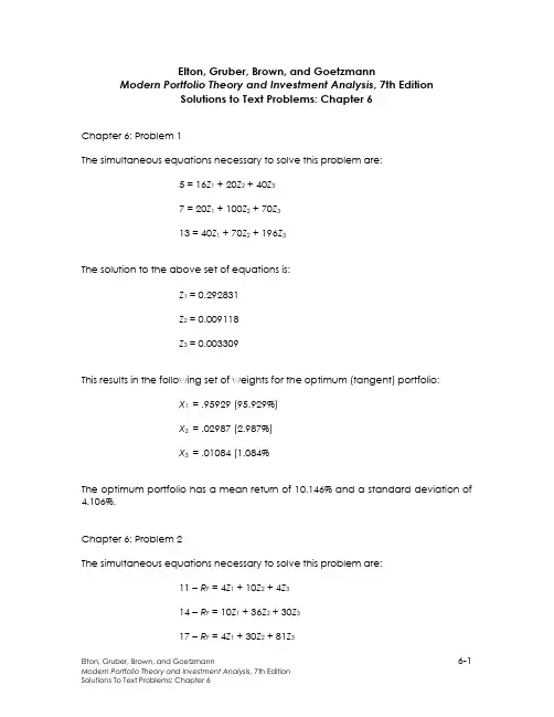
Elton, Gruber, Brown, and GoetzmannModern Portfolio Theory and Investment Analysis, 7th EditionSolutions to Text Problems: Chapter 6Chapter 6: Problem 1The simultaneous equations necessary to solve this problem are:5 = 16Z1 + 20Z2 + 40Z37 = 20Z1 + 100Z2 + 70Z313 = 40Z1 + 70Z2 + 196Z3The solution to the above set of equations is:Z1 = 0.292831Z2 = 0.009118Z3 = 0.003309This results in the following set of weights for the optimum (tangent) portfolio:X1 = .95929 (95.929%)X2 = .02987 (2.987%)X3 = .01084 (1.084%The optimum portfolio has a mean return of 10.146% and a standard deviation of 4.106%.Chapter 6: Problem 2The simultaneous equations necessary to solve this problem are:11 -R F = 4Z1 + 10Z2 + 4Z314 -R F = 10Z1 + 36Z2 + 30Z317 -R F = 4Z1 + 30Z2 + 81Z3The optimum portfolio solutions using Lintner short sales and the given values for R F are: R F = 6% R F = 8% R F = 10%Z 1 3.510067 1.852348 0.194631Z 2-1.043624 -0.526845 -0.010070 Z 3 0.348993 0.214765 0.080537 X 1 0.715950 0.714100 0.682350X 2-0.212870 -0.203100 -0.035290 X 3 0.711800 0.082790 0.282350Tangent (Optimum) Portfolio Mean Return 6.105% 6.419% 11.812%Tangent (Optimum) Portfolio Standard Deviation 0.737% 0.802% 2.971%Chapter 6: Problem 3Since short sales are not allowed, this problem must be solved as a quadratic programming problem. The formulation of the problem is:PFP XR R σθ-=maxsubject to:11=∑=Ni iX0≥i X ∀ iChapter 6: Problem 4This problem is most easily solved using The Investment Portfolio software that comes with the text, but, since all pairs of assets are assumed to have the same correlation coefficient of 0.5, the problem can also be solved manually using the constant correlation form of the Elton, Gruber and Padberg “Simple Techniques” described in a later chapter.To use the software, open up the Markowitz module, select “file” then “new” then “group constant correlation” to open up a constant correlation table. Enter the input data into the appropriate cells by first double clicking on the cell to make it active. Once the input data have been entered, click on “optimizer” and then “run optimizer” (or simply cl ick on the optimizer icon). At that point, you can either select “full Markowitz” or “simple method.”If you select “full Markowitz,” you then select “short sales allowed/riskless lending and borrowing” and then enter 4 for both the lending and borrowin g rate and click “OK.” A graph of the efficient frontier then appears. You may then hit the “Tab” key to jump to the tangent portfolio, then click on “optimizer” and then “show portfolio” (or simply click on the “show portfolio” icon) to view and print the composition (investment weights), mean return and standard deviation of the tangent (optimum) portfolio.If instead you select “simple method,” you then select “short sales allowed with riskless asset” and enter 4 for the riskless rate and click “OK.” A table showing the investment weights of the tangent portfolio then appears.Regardless of the method used, the resulting investment weights for the optimum portfolio are as follows:Asset i X i1 -5.999%2 -17.966%3 21.676%4 0.478%5 -29.585%6 12.693%7 -59.170%8 -14.793%9 3.442%10 189.224%Given the above weights, the optimum (tangent) portfolio has a mean return of 18.907% and a standard deviation of 3.297%. The efficient frontier is a positively sloped straight line starting at the riskless rate of 4% and extending through thetangent portfolio (T) and out to infinity:Chapter 6: Problem 5Since the given portfolios, A and B, are on the efficient frontier, the GMV portfolio can be obtained by finding the minimum-risk combination of the two portfolios:31202163620162222-=⨯-+-=-+-=A B B A A B B GMVA X σσσσσ3111=-=GMVA GMVB X XThis gives %33.7=GMV R and %83.3=GMV σAlso, since the two portfolios are on the efficient frontier, the entire efficient frontier can then be traced by using various combinations of the two portfolios, starting with the GMV portfolio and moving up along the efficient frontier (increasing the weight in portfolio A and decreasing the weight in portfolio B). Since X B = 1 - X A the efficient frontier equations are:()()A A B A A A P X X R X R X R -⨯+=-+=18101()()()()A A A A A BA AB A A A P X X X X X X X X -+-+=-+-+=14011636121222222σσσσSince short sales are allowed, the efficient frontier will extend beyond portfolio A and out toward infinity. The efficient frontier appears as follows:。

投资组合分析报告摘要：本文旨在通过对投资组合的分析和评估，为投资者提供有关投资风险和回报的全面信息。

通过使用一系列的分析工具和方法，我们对投资组合进行了定量和定性的评估，并提出了一些策略建议，以帮助投资者最大限度地优化风险和回报的平衡。

1. 引言投资组合管理是一个复杂而且关键的金融活动，它旨在通过将资金分配到不同的资产类别中，实现投资者的财务目标。

一个有效的投资组合应该是多元化的，以减轻单一资产的风险，并为投资者提供长期的可持续回报。

因此，投资组合分析和评估是投资决策的核心。

2. 投资组合的当前状况我们首先对投资组合的当前状态进行了概述，包括资产类别的分配、各资产类别的回报率以及整体风险水平的评估。

通过对比投资组合的回报与市场基准的表现，我们可以初步评估投资策略的有效性。

3. 资产分配和风险控制在这一部分，我们详细讨论了资产分配的重要性以及如何最大程度地减少投资组合的风险。

我们介绍了不同的资产类别，并说明了它们的特点和风险-回报关系。

通过定量分析和现代投资理论的应用，我们可以确定最佳的资产配置比例以及相关的风险控制策略。

4. 投资者的目标和风险承受能力在这一部分，我们讨论了投资者的目标和风险承受能力对投资组合决策的重要性。

通过准确评估投资者的目标和风险偏好，我们可以为其提供最合适的投资组合建议，并为其制定适合的投资策略。

5. 投资组合的绩效评估为了评估投资组合的绩效，我们使用了一系列的指标和方法，如夏普比率、特雷诺比率和信息比率等。

这些评价指标可以帮助投资者判断投资组合的回报是否与其承担的风险相匹配，并与市场基准进行对比。

6. 策略建议基于我们的分析和评估结果，我们提供了一些具体的策略建议，以帮助投资者改善投资组合的绩效。

这些建议涉及到资产分配的优化、投资策略的调整以及风险管理的改进等方面。

结论：通过对投资组合的分析和评估，我们可以帮助投资者更好地理解其投资组合的风险和回报，并为其提供相应的建议。

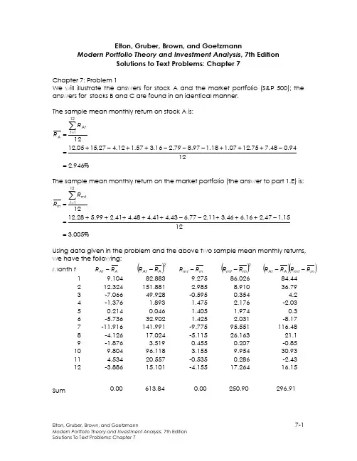
Elton, Gruber, Brown, and GoetzmannModern Portfolio Theory and Investment Analysis , 7th EditionSolutions to Text Problems: Chapter 7Chapter 7: Problem 1We will illustrate the answers for stock A and the market portfolio (S&P 500); the answers for stocks B and C are found in an identical manner.The sample mean monthly return on stock A is:%946.21294.048.775.1207.118.197.879.216.357.112.427.1505.1212121=-+++---++-+==∑=t AtA RRThe sample mean monthly return on the market portfolio (the answer to part 1.E) is:%005.31215.147.216.646.311.277.643.441.448.441.299.528.1212121=-+++--+++++==∑=t m tm RRUsing data given in the problem and the above two sample mean monthly returns, we have the following: Month tAAt R R - ()2AAtR R-mm t R R - ()2mmtR R-()()mm t A AtR R R R--1 9.104 82.883 9.275 86.026 84.442 12.324 151.881 2.985 8.910 36.793 -7.066 49.928 -0.595 0.354 4.2 4 -1.376 1.893 1.475 2.176 -2.03 5 0.214 0.046 1.405 1.974 0.3 6 -5.736 32.902 1.425 2.031 -8.17 7 -11.916 141.991 -9.775 95.551 116.48 8 -4.126 17.024 -5.115 26.163 21.19 -1.876 3.519 0.455 0.207 -0.85 10 9.804 96.118 3.155 9.954 30.93 11 4.534 20.557 -0.535 0.286 -2.43 12-3.886 15.101 -4.155 17.264 16.15Sum0.00613.840.00250.90296.91The sample variance and standard deviation of the stock A’s monthly return are:()15.511284.6131212122==-=∑=t AAtAR Rσ%15.715.51==A σThe sample variance (the answer to part 1.F) and standard deviation of the market portfolio’s monthly return are:()91.201290.2501212122==-=∑=t mm tmR Rσ%57.491.20==m σThe sample covariance of the returns on stock A and the market portfolio is:()()[]74.241291.29612121==--=∑=t mm t A AtAm R R R RσThe sample correlation coefficient of the returns on stock A and the market portfolio (the answer to part 1.D) is:757.057.415.774.24=⨯==mA Am Am σσσρThe sample beta of stock A (the answer to part 1.B) is:183.191.2074.242===mAm A σσβThe sample alpha of stock A (the answer to part 1.A) is:%609.0%005.3183.1%946.2-=⨯-=-=m A A A R R βαEach month’s sample residual is security A’s actual return that month minus the return that month predicted by the regression. The regression’s predic ted monthly return is: mt A A edict ed t A R R βα-=Pr ,,The sample residual for each month t is then: edict ed t A At At R R Pr ,,-=εSo we have the following:Month tAt R edict edt A R Pr,,At ε2At ε112.05 13.92 -1.873.5 2 15.27 6.48 8.79 77.26 3 -4.12 2.24 -6.36 40.45 4 1.57 4.69 -3.12 9.73 5 3.16 4.61 -1.45 2.1 6 -2.79 4.63 -7.42 55.06 7 -8.97 -8.62 -0.35 0.12 8 -1.18 -3.11 1.93 3.72 9 1.07 3.48 -2.41 5.81 10 12.756.68 6.07 36.84 117.48 2.31 5.17 26.73 12 -0.94 -1.97 1.02 1.04Sum: 0.00 262.36Since the sample residuals sum to 0 (because of the way the sample alpha and beta are calculated), the sample mean of the sample residuals also equals 0 and the sample variance and standard deviation of the sample residuals (the answer to part 1.C) are: ()863.211236.26212121211212===-=∑∑==t Att AAtAεεεσε%676.4863.21==A εσRepeating the above analysis for all the stocks in the problem yields: Stock A Stock B Stock Calpha -0.609% 2.964%-3.422%beta 1.183 1.021 2.322correlation with market 0.757 0.684 0.652standard deviation of sample residuals * 4.676% 4.983% 12.341%with %005.3=m R and 91.202=m σ.*Note that most regression programs use N - 2 for the denominator in the sample residual variance formula and use N - 1 for the denominator in the other variance formulas (where N is the number of time series observations). As is explained in the text, we have instead used N for the denominator in all the variance formulas. To convert the variance from a regression program to our results, simply multiply the variance by eitherNN 2- orNN 1-.Chapter 7: Problem 2 A. A.1portfolio from Problem 1 we have:%946.2005.3183.1609.0=⨯+-=A RSimilarly:%032.6=B R ; %556.3=C RThe Sharpe single-index model's formula for a security's variance of return is:2222i m i i εσσβσ+=Using the beta and residual standard deviation for stock A along with the variance of return on the market portfolio from Problem 1 we have:14.51676.491.20183.1222=+⨯=A σSimilarly: 62.462=b σ; 0.2652=c σ A.2From Problem 1 we have:%946.2=A R ; %031.6=B R ; %554.3=C R15.512=A σ; 61.462=B σ; 0.2652=C σ B. B.1According to the Sharpe single-index model, the covariance between the returns on a pair of assets is:2m j i ij SIM σββσ=Using the betas for stocks A and B along with the variance of the market portfolio from Problem 1 we have:254.2591.20021.1183.1=⨯⨯=AB SIM σSimilarly:433.57=AC SIM σ; 568.49=BC SIM σThe formula for sample covariance from the historical time series of 12 pairs of returns on security i and security j is:()()12121∑=--=t j jt i itij R R R RσApplying the above formula to the monthly data given in Problem 1 for securities A, B and C gives:462.18=AB σ; 618.61=AC σ; 085.54=BC σ C. C.1Using the earlier results from the Sharpe single-index model, the mean monthly return and standard deviation of an equally weighted portfolio of stocks A, B and C are:%18.4%556.331%032.631%946.231=⨯+⨯+⨯=P R%348.857.493143.573125.253120.2653162.463115.5131222222=⎪⎪⎭⎫⎝⎛⨯⎪⎭⎫⎝⎛+⨯⎪⎭⎫ ⎝⎛+⨯⎪⎭⎫ ⎝⎛⨯+⨯⎪⎭⎫ ⎝⎛+⨯⎪⎭⎫ ⎝⎛+⨯⎪⎭⎫ ⎝⎛=P σ C.2Using the earlier results from the historical data, the mean monthly return and standard deviation of an equally weighted portfolio of stocks A, B and C are:%18.4%554.331%031.631%946.231=⨯+⨯+⨯=P R%374.808.543162.613146.183120.2653162.463115.5131222222=⎪⎪⎭⎫⎝⎛⨯⎪⎭⎫ ⎝⎛+⨯⎪⎭⎫ ⎝⎛+⨯⎪⎭⎫ ⎝⎛⨯+⨯⎪⎭⎫⎝⎛+⨯⎪⎭⎫ ⎝⎛+⨯⎪⎭⎫ ⎝⎛=P σThe slight differences between the answers to parts A.1 and A.2 are simply due to rounding errors. The results for sample mean return and variance from either the Sharpe single-index model formulas or the sample-statistics formulas are in fact identical.The answers to parts B.1 and B.2 differ for sample covariance because the Sharpe single-index model assumes the covariance between the residual returns of securities i and j is 0 (cov(εi εj ) = 0), and so the single-index form of sample covariance of total returns is calculated by setting the sample covariance of the sample residuals equal to 0. The sample-statistics form of sample covariance of total returns incorporates the actual sample covariance of the sample residuals.The answers in parts C.1 and C.2 for mean returns on an equally weighted portfolio of stocks A, B and C are identical because the Sharpe single-index model formula for the mean return on an individual stock yields a result identical to that of the sample-statistics formula for the mean return on the stock.The answers in parts C.1 and C.2 for standard deviations of return on an equally weighted portfolio of stocks A, B and C are different because the Sharpe single-index model formula for the sample covariance of returns on a pair of stocks yields a result different from that of the sample-statistics formula for the sample covariance of returns on a pair of stocks.Chapter 7: Problem 3Recall from t he text that the Vasicek technique’s forecast of security i ’s beta (2i β) is:121212112121212i i i i i βσσσβσσσβββββββ⨯++⨯+=where 1β is the average beta across all sample securities in the historical period (in this problem referred to as the “market beta”), 1i β is the beta of security i in thehistorical period, 21βσ is the variance of all the sample securities’ betas in the historical period and 21i βσ is the square of the standard error of the estimate of betafor security i in the historical period.If the standard errors of the estimates of all the betas of the sample securities in the historical period are the same, then, for each security i , we have:a i =21βσ where a is a constant across all the sample securities.Therefore, we have for any security i :()111212112121i i i X X aa aβββσσβσββββ-+=⨯++⨯+=This shows that, under the assumption that the standard errors of all historical betas are the same, the forecasted beta for any security using the Vasicek technique is a simple weighted average (proportional weighting) of 1β (the “market beta”) and 1i β (the security’s historical beta), where the weights are the same for each security.Chapter 7: Problem 4Letting the historical period of the year of monthly returns given in Problem 1 equal 1 (t = 1), then the forecast period equals 2 and the Blume forecast equation is:1260.041.0i i ββ+=Using the earlier answer to Problem 1 for the estimate of beta from the historical period for stock A along with the above equation we obtain the stock’s forecasted beta:120.1183.160.041.060.041.012=⨯+=+=A A ββSimilarly:023.12=B β; 803.12=C βChapter 7: Problem 5 A.%4.13=B R ; %4.7=C R ; %2.11=D R B.σ2B = 43.25; σ2C = 20; σ2D = 36.25 C.σAC = 30; σAD = 33.75; σBC = 26; σBD = 29.25; σCD = 18Chapter 7: Problem 6 A.Recall that the formula for a portfolio's beta is: i N is the number of assets in the portfolio.Since there are four assets in Problem 5, N = 4 and X i equals 1/4 for each asset in。