Radioss Step by Step 教程之1：线性静力分析

机械基础杆件的静力分析1. 引言在机械领域中，杆件是一种常见的结构元素，用于构建各种机械装置。

静力分析是对杆件在静力作用下的力学性能进行分析和计算的过程。

本文将介绍机械基础杆件的静力分析方法，包括受力分析、应力分析和变形分析。

2. 受力分析在进行静力分析之前，首先需要进行受力分析，确定杆件上受到的外力和内力。

外力可以是来自其他结构物的载荷，也可以是外部施加的力或力矩。

内力则是由于外力作用而在杆件内部产生的应力引起的。

通过受力分析，可以获得各个杆件的受力情况，为后续的应力分析和变形分析提供依据。

3. 应力分析应力分析是静力分析中的重要环节。

通过对杆件内部的应力进行分析，可以确定杆件是否能够承受外力载荷，以及破坏的可能性。

应力分析包括两个方面：正应力和剪应力的计算。

正应力是指沿着杆件截面法线方向的应力，而剪应力则是沿着截面平面方向的应力。

常用的应力计算方法包括静力学平衡条件和材料力学方程。

3.1 正应力的计算正应力的计算通常采用静力学平衡条件。

根据平衡条件，杆件上各点的合力和合力矩为零。

通过求解这些方程，可以得到各点处的正应力分布。

此外，还需要考虑杆件的几何形状，以及材料的弹性模量和截面面积等参数。

正应力的计算公式如下：σ = F / A其中，σ是正应力，F是受力，A是截面面积。

3.2 剪应力的计算剪应力的计算也采用静力学平衡条件。

剪应力可以通过应力矢量的分解得到。

假设剪应力的作用平面为x-y平面，剪应力的计算公式如下：τ = F / A其中，τ是剪应力，F是受力，A是截面面积。

4. 变形分析变形分析是对杆件在受力作用下产生的变形进行分析和计算的过程。

变形分析的目的是确定杆件的位移和变形程度，评估其结构稳定性。

常用的变形计算方法包括位移方法和位移曲线法。

4.1 位移方法位移方法是根据杆件的几何形状和受力情况，通过求解位移方程来计算杆件的位移量。

位移方程的求解需要考虑杆件的几何形状、材料的弹性模量和截面惯性矩等参数。

4）建立几何模型
•建立关键点1，2 >Modeling>Create >Keypoints >In Active CS 在Keypoint number输入1， Location in active CS输入（0，0， 0），并单击 “Apply”； 在Keypoint number输入2， Location in active CS输入（1，0， 0），并单击 “Apply”； 在Keypoint number输入3， Location in active CS输入（2，0，
2）分析类型（ANTYPE)
选择静力分析，路径：
Main Menu>Solution>-Analysis Type-New Analysis>Static 3）大变形响应(NLGEOM)
如果分析大变形，选择ON。
4）应力刚化效应（SSTIF) 当小变形分析，应力明显地增加或降低结构的刚度时，选择“ON” 5）预应力计算（PSTRES) 如：在垂直压力下的薄园壳或大变形分析要求收敛时应选择 “ON”。 如果想在同一模型上进行预应力分析，选择“ON” 6) 牛顿-拉普森选项（NROPT)
7）划分网格
•GUI:Main Menu>Preprocessor>Meshing>MeshTool •单击Lines 右侧的Set;
•出现 Elment Size on Picked选择框;
•选择线条L1; •单击OK.
•出现Elment Size on Picked lines对话框;
•在NDIV输入4； •单击OK;
3）定义材料特性
•GUI: Main Menu>Preprocessor>Material Props>Material Models；

ANSYS静力分析的简单步骤第一步，启动工作台软件，然后选择与启动DS模块弹出得界面。

第二步，导入三维模型。

根据操作步骤进行。

首先，单击“几何体”，选择“文件”，然后选择弹出窗口中的3D模型文件，如果当时catia文件格式不符，可以把三维图先转换为“.stp”的格式，即可导入。

第三步，选择零件材料：文件导入软件后，在这个时候，依次选择“几何”下的“零件”，并且在左下角的“Details of ‘Part’”中以调整零件材料属性，本次钟形壳的材料是刚。

第四步，划分网格：选择“Project”树中的“Mesh”，右键选择“Generate Mesh”即可在这一点上，你可以在左下角的“网格”对话框的细节调整网格的大小（体积元）。

第五步，添加类型分析：第一选择顶部工具栏上的“分析”按钮，添加需要的类型分析，因为我们需要做的是在这种情况下的静态分析。

所以选择结构静力。

第六步，添加固定约束：首先选择“Project”树中的“Static Structural”按钮，右键点击支持插入固定树。

这时候在左下角的“Details of ‘Fixed Support’”对话框中“Geometry”会被选中，会要求输入固定的支撑面。

在这种情况下，固定支架的类型是表面支持，确定六凹面（此时也可点击“Edge”来确定“边”）。

然后一直的按住“CTRL”键，连续选择其它几个弧面为支撑面，在点击“Apply”进行确认，第七步，添加载荷：选择“Project”树中的“结构静力”，右键选择“Insert”中的“Force”，然后在选择载荷的作用面，再次点击“Apply”按钮进行确定。

第八步，添加变形：右键点击选择“Project”树中的“Solution”，随后依次选择插入，变形，Total”，添加变形。

第九步，添加等效应变：右键单击“项目”的树，“>插入应变->解决方案->添加等效，等效应变。

第十步，添加等效应力：首先右键点击“Project”树中的“Solution—>Insert—> Stress—>Equivalent”，添加等效应力。

m i d a s C i v i lm i d a s C i v i lm i d a s C i v i l图2.8.38 基于位移设计法的结构抗震性能评价m i d a s C i v i l示。

m i d a s C i v i lm i d a s C i v i lm i d a s C i v i lm i d a s C i v i lm i d a s C i v i lm i d a s C i v i lm i d a s C i v i lm i d a s C i v i lm i d a s C i v i lm i d a s C i v i lm i d a s C i v i l1n λ- : 前一步骤(n-1)的荷载因子1λ : 第1荷载步的荷载因子nstep : 总步骤数i : 等差增量步骤号当前步骤的外力向量如下。

0n n λ=⋅P P(10)(3) 第3阶段: 最终步骤的荷载增量(n nstep =) 最终荷载步骤(nstep )的外力向量如下、0nstep nstep λ=⋅P P ; 1.0nstep λ= (11)图2.8.43 自动调整荷载步长的例题(荷载因子结果)m i d a s C i v i l2. 点击步长控制选项 > 增量控制函数定义步长控制函数m i d a s C i v i lm i d a s C i v i lm i d a s C i v i lm i d a s C i v i lm i d a s C i v i lm i d a s C i v i lm i d a s C i v i lm i d a s C i v i lm i d a s C i v i lm i d a s C i v i lm i d a s C i v i lm i d a s C i v i lm i d a s C i v i lm i d a s C i v i lm i d a s C i v i lm i d a s C i v i lm i d a s C i v i lm i d a s C i v i lm i d a s C i v i lm i d a s C i v i lm i d a s C i v i lm i d a s C i v i lm i d a s C i v i lm i d a s C i v i lm i d a s C i v i lm i d a s C i v i lm i d a s C i v i lm i d a s C i v i lm i d a s C i v i lm i d a s C i v i lm i d a s C i v i lATC-40中对不同结构响应类型规定了谱折减系数的下限值(参见表2.8.7)。

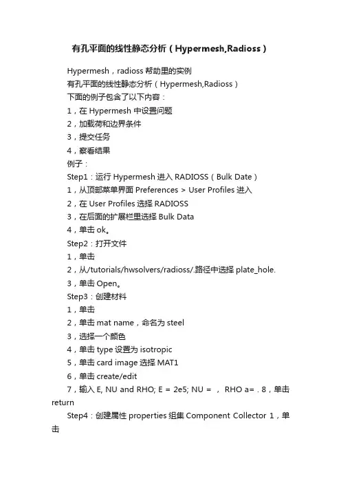
有孔平面的线性静态分析（Hypermesh,Radioss）Hypermesh，radioss帮助里的实例有孔平面的线性静态分析（Hypermesh,Radioss）下面的例子包含了以下内容：1，在Hypermesh 中设置问题2，加载荷和边界条件3，提交任务4，察看结果例子：Step1：运行Hypermesh进入RADIOSS（Bulk Date）1，从顶部菜单界面Preferences > User Profiles进入2，在User Profiles选择RADIOSS3，在后面的扩展栏里选择Bulk Data4，单击ok。

Step2：打开文件1，单击2，从/tutorials/hwsolvers/radioss/.路径中选择plate_hole.3，单击Open。

Step3：创建材料1，单击2，单击mat name，命名为steel3，选择一个颜色4，单击type设置为isotropic5，单击card image选择MAT16，单击create/edit7，输入E, NU and RHO; E = 2e5; NU = ， RHO a= . 8，单击returnStep4：创建属性properties组集Component Collector 1，单击2，单击prop name输入plate_hole3，选择一个颜色4，type选2D5，card image 选PSHELL6，material 选steel7，单击create/edit8，单击[T]输入为平面壳厚度9，单击return10，单击11，单击comps选plate_hole12,将转换成property13，单击property选择plate_hole14,单击update15，单击returnStep5：创建载荷集（spcs和forces）1，单击2，单击loadcol name输入spc3，选颜色4，单击creation method并选择no card image6，单击create7，单击loadcol name输入forces8，单击color选颜色9，单击create10，单击returnStep6：创建约束1，从Model Browser中将LoadCollectors点开，选择建好的spcs右键然后选择Make current使spcs作为当前工作层2，进入Anslysis面板，进入constraints（约束）子面板3，选择nodes，通过节点施加约束4，单击nodes，（鼠标先不要移动），弹出面板后，选择第一个by window，手动画出一个选择区域选取下图所示节点5，选择interior保证框选区域内部节点被选取，单击select entities。

3． 选 BCs > Create > Constraints 创建单点约束。这些约束会固定不允许动的自由度。 4． 在 RADIOSS 里，杆单元是空间单元，有三个自由度 (Ux, Uy, 和 Uz). 为了复制第一部分简单模型，
我们需要消除所有 Uy，Uz 自由度和节点 1 上的 Ux 自由度。在 Constraints 面板里，选节点 1，然后只选 dof1， dof2，dof3。
2. Name 输入 force。在 SPC 方框内打勾，然后点击 = 再选载荷集 SPC. 在 LOAD 方框内打勾，点击 = 然后选载荷集 Force。
3. 确认 type 选的是 linear static 然后选 create。 这就会在 Model Browser 里创建一个新的组叫 Loadstep，包括载荷集 force。
8. 重复这个过程，创建第二部件 A2，选 PROD 属性，面积等于 78.54。也指定 steel 材料。记得把部件 选成另外颜色。
创建这两个部件以后，应该可以在 Model Browser 里看到两个叫 Component 和 Assembly Hierarchy 的新 组，两个里面都有 A1 和 A2。
XI 线性静态分析
本章部分内容来自《Practical Finite Element Analysis》。Debdatta Sen 和 Matthias Goelke 检查 并添加了部分内容。
11.1 线性静态分析
软件根据这个路曲线
应变
线性 线性表示材料线性弹性行为。也就是说，应力-应变曲线的线性部分，一个直线按照胡克定律：σ=εE。这
3. 点击 Property tab, 选择 assign property. Name 输入 A1，card image 选 PROD，选 Create property 就可以设定属性卡片。

➢ 记住关于线性静态结构分析的假设是很重要的。非线性静态分析和动态分析 在后面章节讲解。
第2页/共49页
A. 几何模型
➢ 在结构分析中，可能模拟各种类型的实体。 ➢ 对于面实体，在Details of surface body中
一定要指定厚度值。
第3页/共49页
… 质量点
➢ 在模型中添加一个质量点来模拟结构中没有明确建模的重量体：
Surface Body Face (Scope = Target)
Bonded, No Separation Bonded, No Separation Bonded, No Separation Bonded only
Augmented Lagrange,
All formulations
All formulations
MPC formulation
Symmetry respected
Not supported for solving1
Asymmetric only Bonded only Augmented Lagrange, Pure Penalty, and MPC formulation
Asymmetric only
All formulations
Pure Penalty, and MPC
formulation
Symmetry respected Asymmetric only Surface Body Edge Not supported for solving1 Bonded only
(Scope = Target)
线性静态结构分析基础
➢ 对于一个线性静态结构分析（ Linear Static Analysis ），位移{x}由下面的矩 阵方程解出：

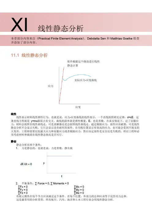
线性静力学分析实例线性静力学问题是简单且常见的有限元分析类型，不涉及任何非线性（材料非线性、几何非线性、接触等），也不考虑惯性及时间相关的材料属性。

在ABAQUS 中，该类问题通常采用静态通用（Static，General）分析步或静态线性摄动（Static，Linear perturbation）分析步进行分析。

线性静力学问题很容易求解，往往用户更关系的是计算效率和求解效率，希望在获得较高精度的前提下尽量缩短计算时间，特别是大型模型。

这主要取决于网格的划分，包括种子的设置、网格控制和单元类型的选取。

在一般的分析中，应尽量选用精度和效率都较高的二次四边形/六面体单元，在主要的分析部位设置较密的种子；若主要分析部位的网格没有大的扭曲，使用非协调单元（如CPS4I、C3D8I）的性价比很高。

对于复杂模型，可以采用分割模型的方法划分二次四边形/六面体单元；有时分割过程过于繁琐，用户可以采用精度较高的二次三角形/四面体单元进行网格划分。

一悬臂梁的线性静力学分析1.1 问题的描述一悬臂梁左端受固定约束，右端自由，结构尺寸如图1-1所示，求梁受载后的Mises应力、位移分布。

ν材料性质：弹性模量32e=E=，泊松比3.0均布载荷：Mpap6.0=图1-1 悬臂梁受均布载荷图1.2 启动ABAQUS启动ABAQUS有两种方法，用户可以任选一种。

（1）在Windows操作系统中单击“开始”--“程序”--ABAQUS 6.10 -- ABAQUS/CAE。

（2）在操作系统的DOS窗口中输入命令：abaqus cae。

启动ABAQUS/CAE后，在出现的Start Section（开始任务）对话框中选择Create Model Database。

1.3 创建部件在ABAQUS/CAE顶部的环境栏中，可以看到模块列表：Module：Part，这表示当前处在Part（部件）模块，在这个模块中可以定义模型各部分的几何形体。

精品jing
3结构线性静力分析
3.结构线性静力分析
3.1静力分析概述
结构分析与结构线性静力分析一般可以分为4个基本步 骤：
建立模型和划分网格 添加载荷和约束 求解 后处理
3.结构线性静力分析
3.2实例分析
3.2.1平面桁架[1] 3.2.2梁[1] 3.2.3井式斜梁格的分析[5] 3.2.4板[1] 3.2.5膜结构[2] 3.2.6受函数荷载的轴承[1] 3.2.7壳-轴对称模型[2] 3.2.8实体
3.2.7壳-轴对称模型[2]
Booleans
Overlap
Delete
LineFillet Booleans
Subtract
Booleans
Add
3.2.8工业厂房的牛腿-实体[4]
E=3e4Mpa,v=0.2 Den=2500kg 单元:solid45,plane42
3.2.8工业厂房的牛腿-实体[4]
3.3小结
Thank you
3.2.4板[1]
如图7—12所示的平面钢板，板厚0.01m，左端固定， 右端作用50kPa的均布荷载。试对其进行静力分析。 弹性横量为210GPa，泊松比为0.25。
单元Plane82
3.2.4板[1]
3.2.4板[1]
PLANE82 Input Summary
Nodes I, J, K, L, M, N, O, P
Body Loads Temperatures -- T(I), T(J), T(K), T(L), T(M), T(N), T(O), T(P)
3.2.5膜结构[2]
模型尺寸
Lx=3m Ly=4m Lz=10mm
物理参数
弹性模量E＝200GPs 泊松比0.3

第18页/共31页
多工况应用
问题大小合并的自由度个数和工况个数决定了“问题大小”。多工况分析可能需要更多的：内存（相对于等效的多步骤分析）。在回代的过程中，方程的右手边必须保留在内存中。硬盘空间（单元和节点数据库）。在可能的情况下，设置：standard_memory 为最小的 I/O (请察看数据文件)。standard_memory_policy 为 MAXIMUM。如果必要，将不同的工况散布到几个分析步中，用以减小每个分析步中内存和硬盘的使用量。 最坏情况：回到多摄动步分析（在这里，还可以比较数据文件中的求解器信息）。
执行： 751 751 模型的细节
相对 CPU 时间 – 3.4 M variable case
8 Steps/8 Load cases
16 Steps/16 Load cases
Solver
7.52
14.3
Total
5.04
7.48
第26页/共31页
例子
修改 501 501 模型8 工况在每个工况中改变对边的边界条件相对全部 CPU 时间： ~0.153
第10页/共31页
线性静态分析和多工况
Multiple *LOAD CASE
Multiple STEP, PERTURBATION
(stiffness/multiple RHS)
(with possibly multiplesmall factorizations)
(simultaneousrecovery)
第12页/共31页
线性静态分析和多工况
三个工况连接件非常柔软，工具上的载荷没有明确指出，但是可能是多种不同类型载荷的组合。
第13页/共31页
多工况应用

如何使用CAD进行线性静力分析CAD软件是一种广泛应用于机械设计领域的工具，它允许工程师们创建、编辑和分析各种类型的图纸和模型。

在设计中，静力学分析是一个重要的环节，它用于评估设计的结构的静态行为和强度。

本教程将介绍如何使用CAD软件进行线性静力学分析。

首先，打开CAD软件并创建一个新的工程文件。

接下来，在绘图界面上选择合适的测量单位，这将决定我们在后续制图和分析过程中所用的单位。

然后，开始绘制模型。

根据设计需求，使用CAD软件的绘图工具创建所需的几何形状。

确保使用准确的尺寸和比例来绘制模型，这将对后续的分析结果产生重要影响。

完成绘图后，我们需要给模型添加约束和加载条件以进行分析。

约束是指限制模型自由度的条件，例如固定支座或约束运动。

加载条件是指施加在模型上的力或压力，例如重力、外部力或约束。

在CAD软件中，我们可以使用不同工具来添加约束和加载条件。

通常情况下，约束可以通过设置特定点的绝对坐标或定义点之间的相对移动来实现。

加载条件可以通过施加所需力或压力的数值来实现。

一旦添加了约束和加载条件，我们就可以开始进行线性静力学分析。

在CAD软件中，这通常通过选择相应的分析功能来实现。

根据不同的软件，操作步骤可能会有所不同，但基本原理是相似的。

在进行分析之前，我们需要选择适当的材料属性和截面特性。

这些属性将在分析过程中用于计算应力和变形。

确保选择准确的材料属性和截面特性对于得到准确的分析结果至关重要。

开始分析后，CAD软件将根据我们提供的约束、加载条件和模型几何来计算模型的应力和变形。

计算过程可能需要花费一些时间，具体取决于模型的复杂性和计算机性能。

完成分析后，我们可以查看模型的结果。

CAD软件通常会提供各种分析结果，包括应力分布、变形图和因子安全系数。

这些结果可以帮助我们评估设计的结构的强度和稳定性。

根据分析结果，我们可以进行必要的修改和优化，以满足设计要求和规范要求。

这可以包括改变材料选择、增加结构支撑或调整模型几何。

Linear Static Analysis of a Plate with a Hole - RD-1000This tutorial demonstrates how to create finite elements on a given CAD geometry of a plate with a hole, apply boundary conditions, and perform a finite element analysis of the problem. Post-processing tools will be used in HyperView to determine deformation and stress characteristics of the loaded plate.The following exercises are included:•Setting up the problem in HyperMesh•Applying Loads and Boundary Conditions•Submitting the job•Viewing the resultsExerciseStep 1: Launch HyperMesh and set the RADIOSS (Bulk Data) User Profileunch HyperMesh.A User Profiles… Graphic User Interface (GUI) will appear. If it does not appear, go to Preferences>User Profiles … from the menu on the top.2.Select RADIOSS in the User Profile dialog.3.From the extended list, select Bulk Data.4.Click OK.This loads the User Profile. It includes the appropriate template, macro menu, and import reader, paring down the functionality of HyperMesh to what is relevant for generating models in Bulk Data Format for RADIOSS and OptiStruct.Step 2: Open the File plate_hole.hm1.Click the Open .hm file icon .An Open file… browser window pops up.2.Select the plate_hole.hm file, located in the HyperWorks installation directory under<install_directory>/tutorials/hwsolvers/radioss/.3.Click Open.The plate_hole.hm database is loaded into the current HyperMesh session, replacing any existing data. The database only contains geometric data.Setting Up the Problem in HyperMeshWhen building models, we encourage you to create the material and property collectors before creating the component collectors. This is the most efficient way of setting up the file since components need to reference materials and properties.Step 3: Create the material1.Click the Material Collector Panel toolbar button .2.Make sure the create subpanel is selected using the radio buttons on the left-hand side of the panel.3.Click mat name = and enter steel.4.Select the desired color for the material steel by clicking on .5.Click type = and select ISOTROPIC.6.Click card image = and select MAT1.7.Click create/edit.The MAT1 card image pops up.If a material property in brackets does not have a value below it, it is off. To edit these materialproperties, click the property in brackets you wish to edit and an entry field will appear below it. Click the entry field and enter a value.8.Enter the following values for E, NU and RHO; E as 2e5; NU as 0.3 and RHO as 7.9e-09.9.Click return twice.A new material, steel, has been created. The material uses RADIOSS's linear isotropic material model,MAT1. This material has a Young's Modulus of 2E+05 and a Poisson's Ratio of 0.3. It is not necessary to define a density value since only a static analysis will be performed. Density values are required,however, for other solution sequences.At any time, the card image for this collector can be modified using the Card Editor .Step 4: Create the properties and update the Component Collector1.Click Properties toolbar icon .2.Make sure the create subpanel is selected using the radio buttons on the left-hand side of the panel.3.Click prop name = and enter plate_hole.4.Select the desired color for the property plate_hole by clicking on .5.Click type = and select 2D.6.Click card image = and select PSHELL.7.Click material = and select steel.8.Click create/edit.The PSHELL card image pops up.9.Click [T] and enter 10.0 as the thickness of the plate.10.Click return twice and go back to the main menu.The property of the shell structure has been created as 2D PSHELL. Material information is also linked to this property.11.Click the Component Collector Panel toolbar button .12.Make sure the update subpanel is selected using the radio buttons on the left-hand side of the panel.13.Click comps >> and select plate_hole from the list.14.Toggle <no property> to property =.15.Click property = twice and select the plate_hole property from the list.Property card image and material information are listed below the property entry field.16.Click update.17.Click return to go to the main menu.The component plate_hole has been updated with a property of the same name and is currently the“Current Component” (see the box in the lower right for plate_hole ). This component uses theplate_hole property definition with a thickness value of 10.0. The material steel is referenced by this component.At any time, the card image for this collector can be modified using the Card Editor and the material referenced by this component collector can be changed using the update option in the Collectors panel.Apply loads and boundary conditions to the modelIn the following steps, the model is constrained so that two opposing edges of the four external edges cannot move. The other two edges remain unconstrained. A total load of 1000N is applied at the edge of the hole in the positive z-direction.Step 5: Create load collectors (spcs and forces )A new load collector, spcs is created.A new load collector, forces is created.Step 6: Create constraints1.Click the Load Collectors toolbar icon .2.Make sure the create subpanel is selected using the radio buttons on the left-hand side of the panel.3.Click loadcol name = and enter spcs .4.Click color and select a color from the color palette.5.Click the creation method switch and select no card image from the pop-up menu.6.Click create .7.Click loadcol name = and enter forces .8.Click color and select a different color from the color palette.9.Click create .10.Click return to go to the main menu.1.From Model Browser expand LoadCollectors , right-click on spcs and click Make current to set spcsas the current load collector.The window is polygonal, and every mouse click creates a window vertex.Illustration of which nodes to select for applying single point constraints. Dofs with a check will be constrained while dofs without a check will be free.Dofs 1, 2, and 3 are x, y, and z translation degrees of freedom.Dofs 4, 5, and 6 are x, y, and z rotational degrees of freedom.This applies these constraints to the selected nodes.Step 7: Create forces on the nodes around the holeThe window is polygonal, and every mouse click creates a window vertex.2.From the Analysis page,enter the constraints panel.3.Make sure the create subpanel is selected using the radio buttons on the left-hand side of the panel.4.Make sure nodes are selected from the entity selection switch.5.Click nodes and select by window from the pop-up extended entity selection menu.6.Draw a window in the graphics area encompassing the nodes to be selected (shown in the figure).7.Check the box beside interior and click on select entities .8.Constrain dof1, dof2, dof3, dof4, dof5, and dof6 and set all of them to a value of 0.0.9.Ensure the load types is set to SPC .10.Click create .11.Click return to go to the main menu.1.Set your current load collector to forces in Model Browser as shown before in point 1 under Step 6.2.From the Analysis page, enter the forces panel.3.Make sure the create subpanel is selected using the radio buttons on the left-hand side of the panel.4.Make sure nodes are selected from the entity selection switch.5.Click nodes and select by window from the pop-up extended entity selection menu.6.Draw a window in the graphics window encompassing the nodes shown in the figure below.Nodes selected for creating loading around hole.7.Check the box beside interior and click on select entities.8.Set the coordinate system toggle to global system.9.Click the vector definition switch and select constant vector.10.Click magnitude = and enter 21.277 (i.e. 1000 divided by the number of nodes 47).11.Click the direction definition switch below magnitude=, and select z-axis from the pop-up menu.12.Ensure the load types is set to FORCE.13.Click create.This creates a number of point forces, with the given magnitude in the z-direction, to be applied to the nodes about the hole.14.Click return to go to the main menu.Step 8: Create a RADIOSS subcase (also referred to as a loadstep)1.From the Analysis page, enter the loadsteps panel.2.Click name = and enter lateral force.3.Click the type: switch and select linear static, if it is not already selected by default.4.Check the box preceding SPC.An entry field appears to the right of SPC.5.Click on the entry field and select spcs from the list of load collectors.6.Check the box preceding LOAD.An entry field appears to the right of LOAD.7.Click on the entry field and select forces from the list of load collectors.8.Click create.A RADIOSS subcase has been created which references the constraints in the load collector spcs andthe forces in the load collector forces.9.Click return to go to the main menu.Step 9: Submitting the job1.From the Analysis page, enter the RADIOSS panel.2.Click save as… following the input file: field.A Save file… browser window pops up.3.Select the directory where you would like to write the RADIOSS model file and enter the name for themodel, plate_hole.fem, in the File name: field.The .fem filename extension is the recommended extension for RADIOSS Bulk Data Format input decks.4.Click Save.Note the name and location of the plate_hole.fem file displays in the input file: field.5.Set the export options:toggle to all.6.Click the run options: switch and select analysis.7.Set the memory options: toggle to memory default.8.Click Radioss.This launches the RADIOSS job. If the job is successful, you should see new results files in the directory from which plate_hole.fem was selected. The plate_hole.out file is a good place to look for error messages that could help debug the input deck if any errors are present.The default files written to the directory are:plate_hole.html HTML report of the analysis, giving a summary of the problemformulation and the analysis results.plate_hole.out RADIOSS output file containing specific information on the file setup,the setup of your optimization problem, estimates for the amount ofRAM and disk space required for the run, information for eachoptimization iteration, and compute time information. Review this filefor warnings and errors.plate_hole.h3d HyperView binary results file.plate_hole.res HyperMesh binary results file.plate_hole.stat Summary of analysis process, providing CPU information for eachstep during analysis process.Viewing the ResultsDisplacement and Stress results for linear static analyses are output from RADIOSS by default. The following steps describe how to view those results in HyperView.HyperView is a complete post-processing and visualization environment for finite element analysis (FEA), multi-body system simulation, video and engineering data.Step 10: View a contour plot of stresses1.Once you receive the message 'Process Completed Successfully' in the command window, clickHyperView.HyperView is launched and the results are loaded. A message window appears to inform of thesuccessful model and result files loading into HyperView.2.Click Close to close the message window.3.Click the Contour toolbar button .4.Select the first pull-down menu below Result type:and select Element Stresses [2D & 3D] (t).5.Select the second pull-down menu below Result type:and select vonMises.6.Select None in the field below Averaging method:.7.Click Apply.A contoured image representing von Mises stresses should be visible. Each element in the model isassigned a legend color, indicating the von Mises stress value for that element, resulting from the applied loads and boundary conditions.8.Click Top in the view controls from the bottom right corner to view the model, as shown in the followingfigure.von Mises stress assigned plotWhat is the maximum von Mises stress value?At what location does the model have its maximum stress?Does this make sense based on the boundary conditions applied to the model?Step 11: View a contour plot of displacements1.Select the first pull-down menu below Result type:and select Displacement (v).2.Select the second pull-down menu below Result type:and select Mag.3.Click Apply.The resulting contours represent the displacement field resulting from the applied loads and boundary conditions.What is the maximum Displacement value?At what location does the model have its maximum displacement?Does this make sense based on the boundary conditions applied to the model?Step 12: View the deformed shape1.Click Iso in the view controls (bottom right corner) to display the isometric view of the model.2.Click the Deformed toolbar button .3.Set Result type: to Displacement(v), Scale:to Scale factor; and Type:to Uniform.4.In the field next to value, enter 500.This means that the displacement results of the analysis will be multiplied by 500.5.For Show:, select Wireframe.6.Click Apply.A deformed plot of your model with displacement contour should be visible, overlaid on the originalundeformed mesh. Refer to the following figure to see what the plot should look like in isometric view.Isometric view of deformed plot overlaid on the original undeformed mesh with model units set to 500.Go ToRADIOSS, MotionSolve, and OptiStruct Tutorials。

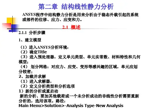
第二章结构线性静力分析2.1静力分析的定义静力分析计算在固定不变载荷作用下结构的响应，它不考虑惯性和阻尼影响，如结构受随时间变化载荷作用的情况。

可是静力分析可以计算那些固定不变的惯性载荷对结构的影响(如重力和离心力)，以及那些可以近似为等价静力作用的随时间变化载荷(如通常在许多建筑规范中所定义的等价静力风载和地震载荷)的作用。

静力分析用于计算由那些不包括惯性和阻尼效应的载荷作用于结构或部件上引起的位移、应力、应变和力。

固定不变的载荷和响应是一种假定，即假定载荷和结构响应随时间的变化非常缓慢。

静力分析所施加的载荷包括：外部施加的作用力和压力稳态的惯性力(如重力和离心力)强迫位移温度载荷(对于温度应变)能流(对于核能膨胀)关于载荷，还可参见§2.3.4。

2.2线性静力分析与非线性静力分析静力分析既可以是线性的也可以是非线性的。

非线性静力分析包括所有类型的非线性：大变形、塑性、蠕变、应力刚化、接触(间隙)单元、超弹性单元等。

本章主要讨论线性静力分析。

对非线性静力分析只作简单介绍。

2.3静力分析的求解步骤2.3.1建模首先用户应指定作业名和分析标题，然后通过PREP7前处理程序定义单元类型、实常数、材料特性、模型的几何元素。

这些步骤是大多数分析类型共同的，并已在《ANSYS Basic Analysis Guide》§1.2论述。

有关建模的进一步论述，见《ANSYS Modeling and Meshing Guide》。

2.3.1.1注意事项在进行静力分析时，要注意如下内容：1、可以采用线性或非线性结构单元。

2、材料特性可以是线性或非线性，各向同性或正交各向异性，常数或与温度相关的：必须按某种形式定义刚度(如弹性模量EX，超弹性系数等)。

对于惯性载荷(如重力等)，必须定义质量计算所需的数据，如密度DENS。

对于温度载荷，必须定义热膨胀系数ALPX。

3、对于网格密度，要注意：应力或应变急剧变化的区域(通常是用户感兴趣的区域)，需要比应力或应变近乎常数的区域较密的网格：在考虑非线性的影响时，要用足够的网格来得到非线性效应。

第6章结构线性静⼒分析第6章结构线性静⼒分析6.1 结构线性静⼒分析概述结构线性静⼒分析的重要性：★结构线性静⼒分析最为常⽤。

★设计规范基本上采⽤线弹性分析结构的内⼒。

★是各种分析的基础。

结构分析的四个基本步骤：◆创建⼏何模型◆⽣成有限元模型◆加载与求解◆结果评价与分析。

6.1.1 创建⼏何模型⑴清除当前数据库①回到开始层：FINISH命令。

清除数据库的操作要在开始层。

②清除数据库：/CLEAR命令。

开始新⼯作前清除数据库。

⑵⼯作⽂件名与主标题①⼯作⽂件名：/FILNAME命令。

建议⽤户定义。

②主标题：/TITLE命令。

⽤于在图形区显⽰。

⼦标题可⽤/STITLE命令定义。

⑶创建具体的⼏何模型6.1.2 ⽣成有限元模型⑴定义单元类型、实常数和材料性质①定义单元类型，设置单元的KEYOPT的选项。

②定义单元实常数，如有初应变时也应设置。

③定义弹性模量，如为各项同性时只需定义EX即可。

④定义质量密度，以便计算⾃重影响或惯性释放计算。

⑤定义热膨胀系数等。

此部分常常在创建具体的⼏何模型之前定义，以便在⼏何模型上施加荷载与约束。

⑵定义⽹格划分属性①定义单元划分数⽬或⼤⼩。

②定义单元划分类型和划分⽅式，如映射⽹格或⾃由⽹格等。

③对⼏何模型实施⽹格划分。

6.1.3 加载与求解⑴定义求解选项①进⼊求解层。

有些荷载可以在前处理层施加，不必⼀定到求解层施加。

②定义分析类型，ANSYS缺省分析类型为静态分析，也可省略。

③定义求解选项，如输出、求解器等选项的设置。

⑵加载①划分荷载步。

②施加约束，约束可在⼏何模型上施加，也可在有限元模型上施加。

③施加荷载，静⼒分析的荷载如集中荷载、分布荷载、温度、⾃重和旋转惯性⼒。

对梁单元的分布荷载必须施加在有限元模型上。

⑶求解6.1.4 结果评价与分析①进⼊通⽤后处理，⼀般不必进⼊时程后处理。

②读⼊结果数据，如确定读⼊哪个荷载步的结果。

③对结果处理，并图形显式和列表显⽰结果。

④误差估计，仅SOLID和SHELL单元可考察⽹格密度对结果的影响。

目录
应用工程实例展示与功能介绍
1. 应用工程实例展示
1. 应用工程实例展示
2. 功能介绍
2. 功能介绍
➢ 线性静力分析 ➢ 非线性单元线性静力分析（非线性单元、非线性边界） ➢ 特征值分析 ➢ 反应谱分析 ➢ 线弹性时程分析 ➢ 屈曲分析 ➢ 几何非线性分析（牛顿-拉普森法、弧长法） ➢
2. 功能介绍
➢ P-Δ 分析 ➢ 边界非线性时程分析 ➢ （粘弹性阻尼器、间隙、钩、滞回系统、铅芯橡胶支座、摩擦摆隔 震装置） ➢ 材料非线性分析 （塑性材料本构模型：特雷斯卡Tresca、范梅塞斯von Mises、 莫尔-库 伦Mohr-Coulomb、德鲁克-普拉格Druker-Prager） ➢ 静力弹塑性分析（ Pushover分析） ➢ （荷载控制法、位移控制法）
1. 建模一般流程
简支梁、连续梁建模操作
前处理
• 定义材料、截面特性 • 建立节点、单元，生成模型 • 添加边界条件 • 施加荷载
分析
• 定义分析控制 • 运行分析
后处理
• 查看一般结果：反力、位移、内力 • 应力（图例、表格、图标） • 设计验算
2跨连续梁建模
前处理
2跨连续梁建模
前处理
2跨连续梁建模
midas Civil 施工专题—万能杆件塔架稳定性
Integrated Solution System for Bridge and Civil Strucutres
分析与钢围堰分析
熟悉软件 1. 应用工程实例展示与功能介绍 2. 简支梁、连续梁建模操作
应用软件 1. 万能杆件塔架稳定性分析 2. 钢围堰建模与分析
N
下，结构发生屈曲。
钢围堰分析
模型

节点1是固定的，所以这个节点位移是零。因此我们可以消除第一行和第一列。
解决这个问题我们需要两侧同乘倒置的整体刚度矩阵。
这就给出了节点2和3的位移值。确定位移矢量以后，就可以确定单元应变、应力和力。 应变
应力
力
这是很简单的例子，可是精心总结了有限元分析在线性静态问题中的使用。以上所有的计算是求解器计算 的。要是用户需要更详细的有限元分析信息，可以在网上文档或者参考书籍中找到。
两个圆：Ri=50 mm; Ra=250 mm。
两圆中间创建填充表面。 然后沿表面法向拉 5mm，形成封闭的 3D 几何。
网格划分 用 Solid Map Mesh 面板创建实体单元。
确定圆盘中心和柱坐标系 模型里需要指定柱坐标系才能计算径向应力和切向应力（Sxx 和 Syy）。
可以用 Distance 面板确定圆盘中心。注意用三节点子面板。 在内圈选三个节点，点击 circle center. 重复上一步，确定另外表面中心。 用这两临时节点确定柱坐标系 z 方向，选 Geometry > Create > Systems > Node Reference。
第三步 创建有限元网格和合适属性 这一步取决于模型。可以从导入的 CAD 几何开始，或者导入另外 FEA 模型，或者这两办法并用。在我们
的例子中，模型很简单，所以可以直接创建节点和单元。 1. 用 F8 快捷键创建节点，会打开 Create Nodes 面板。
2. 创建三个节点在这些坐标：(0,0,0), (100,0,0), 和 (300,0,0)
2． 现在应该在节点 3 创建 X 负方向的力。用 BCs > Create > Forces 下面的 Forces 面板。 3． Nodes 选 node3。magnitude 输入-10，然后选 x-axis，具体如下：

毕业论文（设计）任务书学院机械工程学院专业机械设计制造及其自动化班级学生姓名学号指导教师目录摘要Abstract第一章绪论第二章结构线性静力分析过程及实例分析（2）2.1 输气管道受力分析2.1.1 问题描述2.1.2 问题分析2.1.3 求解步骤第三章结构线性静力分析过程及实例分析（1）3.1 带孔波板两端承受均布载荷3.1.1 问题描述3.1.2 问题分析3.1.3 求解步骤结论致谢参考文献第一章结构线性静力分析过程及实例分析（1）1.1 带孔波板两端承受均布载荷1.1.1 问题描述某带孔薄板承载示意图见图1。

薄板中心有一圆孔，在其两端受均布载荷q=1000Pa，求薄板内部的应力场分布（图中单位为mm）。

相关参数：弹性模量E=200Gpa，泊松比=0.3，平均厚度=0.01mm。

图1 薄板承载示意图1.1.2 问题分析该问题属于平面应力问题。

根据平板结构的对称性，选择整体结构的1/4建立几何模型，进行分析求解。

1.1.3 求解步骤1.定义件名和工作标题1）选择Utility Menue→File→Change Jobname命令,出现Change Jobname 对话框,在[/Filnam]Enter New Jobname输出栏中输出工作文件名EXERCISE1,并将New Log And Error Files设置为Yes, 如图3-2所示，单击【Ok】按钮关闭该对话框。

2）选择Utility Menue→File→Change Title命令，出现Change Title对话框，在输出栏中输入ANALYSIS OF PLATE STRESS WITH SMALL CIRCLE，如图3-3所示，单击【Ok】按钮关闭该对话框。

2.定义单元类型1)选择Main Menue→Preprocessor→Element Type→Add/Edit/Delete命令,出现Element Types对话框,单击【Add】按钮，出现Library Of Element Types 对话框。