14等效噪声带宽

等效噪声带宽计算公式
等效噪声带宽计算公式，是用于评估电路或系统中噪声对性能的影响程
度的一种数学模型。

通过计算等效噪声带宽，可以预测噪声信号在电路中的
表现并进行优化设计。

等效噪声带宽计算公式通常用于分析和设计各种通信、电子设备和电路，以确保信号传输过程中的噪声最小化，从而提高系统性能和可靠性。

在模拟
电路和数字电路设计中，等效噪声带宽计算公式被广泛应用。

一种常用的等效噪声带宽计算公式是通过计算信噪比（SNR）来确定。

SNR通常用分贝（dB）表示，计算公式为SNR = 10log10(Psignal/Pnoise)，
其中Psignal代表信号功率，Pnoise代表噪声功率。

等效噪声带宽（ENBW）可以通过以下公式计算得出：
ENBW = (SNR/Signal-to-noise ratio at 1 Hz) * Bandwidth
其中，Signal-to-noise ratio at 1 Hz是信噪比在1 Hz带宽上的值。

这个值
通常可以通过实验或模拟计算得到，并且往往与电路的参数和特性相关。

通过等效噪声带宽计算公式的应用，设计工程师可以估计系统中的噪声
级别，对信号的传输质量和系统的性能进行分析和评估。

在实际应用中，根
据具体的设计要求和系统特性，可以选择合适的噪声模型和计算方法来推导
等效噪声带宽。

总之，等效噪声带宽计算公式是设计电路和系统时必备的工具之一，它
能够帮助工程师估计噪声对系统的影响，从而指导优化设计和提高系统性能。

正确使用和理解等效噪声带宽计算公式，可以在电路设计中发挥重要的作用。

光学噪声常用计算公式整汇总
在光学中，常用的噪声计算公式有以下几种：
1. 光电噪声：光电噪声可以通过夏克定理计算，公式为：NEP = sqrt(2*h*f*P) ，其中NEP为光电噪声等效功率，h为普朗克
常数， f为光频率， P为光功率。

2. 热噪声：热噪声主要包括热涨落噪声和热传导噪声。

热涨落噪声可以通过尼奎斯特定理计算，公式为：N = 4*k*T*R*B ，其中N为噪声功率密度，k为玻尔兹曼常数，T为温度，R为
电阻值，B为等效噪声带宽。

热传导噪声可以通过计算器件的
等效散热电阻来估算。

3. 惯性噪声：惯性噪声主要包括机械振动噪声和气体流动噪声。

机械振动噪声可以通过计算器件的振动谐振频率和阻尼系数来估算。

气体流动噪声主要与器件工作环境中的气体流速和压力变化相关。

4. 量子噪声：量子噪声主要包括黑体辐射噪声和光子统计噪声。

黑体辐射噪声可以通过斯蒂芬—玻尔兹曼定律计算，公式为：
N = sigma * T^4 ，其中N为噪声功率密度，sigma为斯蒂芬—
玻尔兹曼常数，T为温度。

光子统计噪声可以通过计算器件接
收到的平均光子数来估算，公式为：N = sqrt(F * P * h * f) ，
其中N为光子噪声等效功率，F为器件的量子效率，P为光功率，h为普朗克常数，f为光频率。

这些公式是光学噪声计算中常用的公式，可以根据具体的应用场景和噪声来源进行选择和应用。

4-4设有限时间积分器的单位冲激响应h(t)=U(t)－U(t －0.5) 它的输入是功率谱密度为 210V Hz 的白噪声，试求系统输出的总平均功率、交流平均功率和输入输出互相关函数()()()()()22221:()2[()][()]0Y Y Y Y XY X P E Y t G d D Y t E Y t m E Y R R R h ωωπτττ∞-∞⎡⎤==⎣⎦⎡⎤=-==⎣⎦=*⎰思路()()()10()()10()10[()(0.5)]()()10[()(0.5)]XY X YX XY R R h h h U U R R U U τττδτττττττττ=*=*==--=-=----解：输入输出互相关函数()Y R τ00020.025()0()10()10()0()()()()10(()00[()(0.)()10()()()10()()10101100.55[()5)]](0)X X X Y X Y X Y Y X t m G R m m h d R U R h h h h h h d R h h d d d E Y t R U ωτττττττττλτλδτλλλλλλλμ∞∞∞∞==⇔====**-=*-=+=+=-=-=⋅=⨯==⎰⎰⎰⎰⎰时域法平均功是白噪声，，，率面积法：225[()][()]5Y Y D Y t E Y t m ==-=P 交流：平均功率()()()2141224222Y2(P1313711()2415()()()102424115112522242j j j Y X Y U t U t Sa e H e Sa G G H e Sa Sa G d Sa S d a d ωτωωωτττωωωωωωωωωωωππωωπ---∞∞∞-∞∞--∞⎛⎫--⎡⎤ ⎪⎣⎦⎝⎭-⎛⎫⇒= ⎪⎝⎭⎛⎫⎛⎫=== ⎪ ⎪⎝⎭⎝⎭⎛⎫===⎛⎫= ⎪ ⎭⎪⎭⎝⎝⎰⎰⎰P 矩形脉冲A 的频谱等于A 信号与线性系统书式域法）频()()2220000[()][()][()]5Y X Y Y m m H H D Y t E Y t m E Y t =⋅=⋅⇒=-===P 交直流分量为平均功率：流4-5 已知系统的单位冲激响应()(1)[()(1)]h t t U t U t =---，其输入平稳信号的自相关函数为()2()9X R τδτ=+，求系统输出的直流功率和输出信号的自相关函数？分析：直流功率＝直流分量的平方解: 输入平稳输出的直流分量 输出的直流功率()2300X X m R σ==±==()()()10332Y X m m h t h t ττ=*=*=⎰=31-d ()()()()()()()()()()()()()()()2'''222'[()(1()(1)(1)F )]12122222j j j j Y h t t t d F j d d F j jd H A A U t U t A Sa ej A Sa e Sa e Sa eG U t U t t j ωωωωωωωωωωωωωωωωωω----⋅↔⇒⋅↔-⇒=-⎛⎫--⇒=⎡⎤ ⎪⎣⎦⎝⎭⎡⎤⎛⎫⎛⎫⎛⎫⎛⎫⇒==+⋅-⎢⎥ ⎪ ⎪ ⎪ ⎪⎝⎭⎝⎭⎝⎭⎝=-=-⎭⎣-=-⎦变换 频域的微分特性 -jt f t t f t =A t A t 矩形脉冲A 谱t 的频()()()()()()()()()()()2''21920222410001lim 022239024X X Y Y X G H G H H Sa Sa R j H A A j Sa m m H j ωωωωωωωωπδτω*→=⋅⋅⎡⎤⎛⎫⎛⎫=-+⇒ ⎪ ⎪⎢⎥⎝⎭⎝⎭⎣⎦⎛⎫⎛⎫---== ⎪ ⎪⎝⎭⎝⎭=⋅=⇒＝＝直流功率294Y m =()Y X m m h t =*4-7 已知如图4.21 所示的线性系统，系统输入信号是物理谱密度为0N 的白噪声，求：①系统的传递函数()H ω？②输出()Z t 的均方值？其中2222[sin()][()]2ax dx a ax dx axSa π∞∞==⎰⎰()()()()()()()112122121212()()()()()()()()()()()F ()(1)()()11()()()()()()()(()j T Y t X t X t T h t t t T t h t d U t Y X H Y H X H H H H H H e H j H h H t h t H ωωωωωωωωωωωωωωωπδωωωωδδωλδλω-∞-∆∆=--=--⇒=⋅==⇒⇒=-=+=⋅=⋅⋅=⎡⎤⎣⎦⎰Z Z 可以分别求冲激响应，输入为冲激函数：输入为冲激函数、，冲激响应＝1(1)()1)[()](1)()j Tj T j T e e e j j ωωωπδωπδωωω----=-+=-＋()2222222220022022102(2)(1)(1)2()(1cos )2sin sin 2sin ((0)()()()21sin 21sin (0)2)()()()[()]j T j T Z X j Z Z Z Z Z Z e e H T j j T TN T G G H H N T N e d T R G R R F G R N ωωωτωωωωωωωωωωωωωωωωωπωωπωωττω+∞-∞----=⋅=-⋅=⇒⋅=⋅⋅=⋅-⋅⇒⋅==⋅⎰＝＝＝求输出Z t 的均方值即，所以有2200000sin 2222j e d N TN N T d T τωωπωπωπ∞-∞∞=⋅⋅=⋅⋅=⎰⎰4-11 已知系统的输入为单位谱密度的白噪声，输出的功率谱密度为2424()109Y G ωωωω+=++求此稳定系统的单位冲激响应()h t ？解：()()()()()()()()()()()()()()()()()()()()()()242223211242()41092243311()()12231311112()0231921Y t Y X X t G s s s s s s G H G H s H s H s s j H s H s s j j h t F H F e e U t j j s s j s H G s ωωωωωωωωωωωωωωωωω----⋅==⇒=-=++=⇒=++++⎛⎫ ⎪+=++-+-+====+ ⎪++ ⎪⎝⎭-+-+-+==系统稳定，则零头、极点都＋在左半平面带入4-12 已知系统输入信号的功率谱密度为223()8X G ωωω+=+ 设计一稳定的线性系统()H ω，使得系统的输出为单位谱密度的白噪声？解：()()()()()221()11()Y X X G G H s s H s G s H s H ωωωω=⇒⋅=⇒==⇒==即4-14 功率谱密度为02N 的白噪声作用于(0)2H =的低通网络上，等效噪声带宽为XH MHz 。

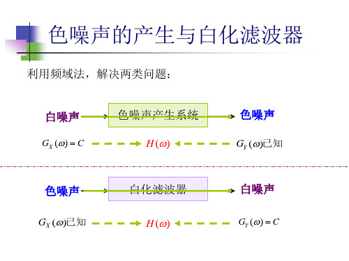
热噪声加性白高斯噪声（AWGN ：Additive White Gaussian Noise ）是最基本的噪声与干扰模型，通信中遇到的多数噪声和干扰都符合这个模型，其中最典型的是热噪声(Thermal Noise)。

一 电阻的热噪声将一个电阻从正中间画一条线分成上下两部分，那么线上的自由电子数和线下的自由电子数的数目是随机的，上下数目差也是随机的。

这个数目差意味着一个电动势，如果有闭合回路的话（如图4.8.2），就会形成一个随机电流，这就是热噪声。

叫热的原因是因为在绝对0度时，电子不运动，这样就不会有随机的电动势。

很显然，电阻的温度越高，随机性也就越强。

每个电子都在随机运动，上下数目差是这些电子随机运动的后果。

电子的总个数足以满足中心极限定律的条件，由此可知热噪声具有高斯的特征。

电子的运动速度极高。

相对于通信中的时间单位如ms 、µs 乃至ns 而言，在极短的一个时间间隔后，上下的电子数目已经毫不相关了，就是说热噪声的自相关函数对于我们的时间刻度来说是一个冲激函数，因此热噪声是一个白噪声。

综合这两点就是说：热噪声是白高斯噪声。

特别注意：白与高斯是两个单独的特征。

高斯是指一维分布，白由二维分布决定。

设()X t 是随机过程，下面的陈述A 涉及一维分布，陈述B 涉及二维分布。

A. 对X(t)进行了大量测试后发现，80%高于4.5，60%高于3.5；B ．对X(t)同时观察相隔10秒的两个值()X t 和()10X t −，大量观察发现，在90%的情况下，()X t 与比10秒前相比，相差不会超过1±V ；在80%的情况下，相差不会超过±0.5V 。

物理学家告诉我们，热噪声的单边功率功率谱密度为0N KT =，其中231.3810K −=×是波尔兹曼常数，T 是绝对温度。

热噪声在带宽B 内的噪声功率KTB （本讲中所谈论的噪声功率均指在匹配负载上的可获功率）。

《微弱信号检测》练习题1、证明下列式子：（1）R xx(τ)=R xx(-τ)（2）∣ R xx(τ)∣≤R xx(0)2x(t)x(t-τ)≤x2(t)+x2(t-τ)∣ R xx(τ)∣≤R xx(0)（3）R xy(-τ)=R yx(τ)（4）| R xy(τ)|≤[R xx(0)R yy(0)]2、设x(t)是雷达的发射信号，遇目标后返回接收机的微弱信号是αx(t-τo)，其中α«1，τo是信号返回的时间。

但实际接收机接收的全信号为y(t)= αx(t-τo)+n(t)。

（1）若x(t)和y(t)是联合平稳随机过程，求R xy(τ)；（2）在（1）条件下，假设噪声分量n(t)的均值为零且与x(t)独立，求R xy(τ)。

3、已知某一放大器的噪声模型如图所示，工作频率f o=10KHz，其中E n=1μV，I n=2nA，γ=0，源通过电容C与之耦合。

请问：（1）作为低噪声放大器，对源有何要求？（2）为达到低噪声目的，C为多少？4、如图所示，其中F1=2dB，K p1=12dB，F2=6dB，K p2=10dB，且K p1、K p2与频率无关，B=3KHz，工作在To=290K，求总噪声系数和总输出噪声功率。

5、已知某一LIA的FS=10nV，满刻度指示为1V，每小时的直流输出电平漂移为5⨯10-4FS；对白噪声信号和不相干信号的过载电平分别为100FS和1000FS。

若不考虑前置BPF的作用，分别求在对上述两种信号情况下的Ds、Do和Di。

6、下图是差分放大器的噪声等效模型，试分析总的输出噪声功率。

7、下图是结型场效应管的噪声等效电路，试分析它的En-In模型。

8、R1和R2为导线电阻，R s为信号源内阻，R G为地线电阻，R i为放大器输入电阻，试分析干扰电压u G在放大器的输入端产生的噪声。

9、如图所示窄带测试系统，工作频率f o=10KHz，放大器噪声模型中的E n=μV，I n=2nA，γ=0，源阻抗中R s=50Ω，C s=5μF。

MT-048TUTORIALOp Amp Noise Relationships: 1/f Noise, RMS Noise,and Equivalent Noise Bandwidth"1/f" NOISEThe general characteristic of op amp current or voltage noise is shown in Figure 1 below.LOG fNOISE nV / √HzorμV / √Hz e n , i n k F CFigure 1: Frequency Characteristic of Op Amp NoiseAt high frequencies the noise is white (i.e., its spectral density does not vary with frequency). This is true over most of an op amp's frequency range, but at low frequencies the noise spectral density rises at 3 dB/octave, as shown in Figure 1 above. The power spectral density in this region is inversely proportional to frequency, and therefore the voltage noise spectral density is inversely proportional to the square root of the frequency. For this reason, this noise is commonly referred to as 1/f noise . Note however, that some textbooks still use the older term flicker noise .The frequency at which this noise starts to rise is known as the 1/f corner frequency (F C ) and is a figure of merit—the lower it is, the better. The 1/f corner frequencies are not necessarily the same for the voltage noise and the current noise of a particular amplifier, and a current feedback op amp may have three 1/f corners: for its voltage noise, its inverting input current noise, and its non-inverting input current noise.The general equation which describes the voltage or current noise spectral density in the 1/f region isf1F k ,i ,e Cn n =, Eq. 1where k is the level of the "white" current or voltage noise level, and F C is the 1/f corner frequency.The best low frequency low noise amplifiers have corner frequencies in the range 1 Hz to 10 Hz, while JFET devices and more general purpose op amps have values in the range to 100 Hz. Very fast amplifiers, however, may make compromises in processing to achieve high speed which result in quite poor 1/f corners of several hundred Hz or even 1 kHz to 2 kHz. This is generally unimportant in the wideband applications for which they were intended, but may affect their use at audio frequencies, particularly for equalized circuits.RMS NOISE CONSIDERATIONSAs was discussed above, noise spectral density is a function of frequency. In order to obtain the rms noise, the noise spectral density curve must be integrated over the bandwidth of interest.In the 1/f region, the rms noise in the bandwidth F L to F C is given by⎥⎦⎤⎢⎣⎡==∫L C C nw F F Cnw C L rms ,n F F ln F v df f 1F v )F ,F (v CLEq. 2where v nw is the voltage noise spectral density in the "white" region, F L is the lowest frequency of interest in the 1/f region, and F C is the 1/f corner frequency.The next region of interest is the "white" noise area which extends from F C to F H . The rms noise in this bandwidth is given byC H nw H C rms ,n F F v )F ,F (v −= Eq. 3Eq. 2 and 3 can be combined to yield the total rms noise from F L to F H :)F F (F F ln F v )F ,F (v C H L C C nw H L rms ,n −+⎥⎦⎤⎢⎣⎡= Eq. 4In many cases, the low frequency p-p noise is specified in a 0.1 Hz to 10 Hz bandwidth, measured with a 0.1 to 10 Hz bandpass filter between op amp and measuring device. The measurement is often presented as a scope photo with a time scale of 1s/div, as is shown in Figure 2 below for the OP213.20nV/div.(RTI)1s/div.Figure 2: 0.1Hz to 10 Hz Input Voltage Noise for the OP213510152025300.1110100FREQUENCY (Hz)INPUT VOLTAGE NOISE, nV / √Hz 0.1Hz to 10Hz VOLTAGE NOISEFor F L = 0.1Hz, F H = 10Hz, v nw = 10nV/√Hz, F C = 0.7Hz:V n,rms = 33nVV n,pp = 6.6 ×33nV = 218nV200nVTIME -1sec/DIV.Figure 3: Input Voltage Noise for the OP177It is possible to relate the 1/f noise measured in the 0.1 to 10 Hz bandwidth to the voltage noise spectral density. Figure 4 above shows the OP177 input voltage noise spectral density on the left-hand side of the diagram, and the 0.1 to 10 Hz peak-to-peak noise scope photo on the right-handV n,rms (F L , F H ) = v nwF C lnF C F L+ (F H –F C )side. Equation 2 can be used to calculate the total rms noise in the bandwidth 0.1 to 10 Hz by letting F L = 0.1 Hz, F H = 10 Hz, F C = 0.7 Hz, v nw = 10 nV/√Hz. The value works out to be about 33 nV rms, or 218 nV peak-to-peak (obtained by multiplying the rms value by 6.6—see the following discussion). This compares well to the value of 200 nV as measured from the scope photo.It should be noted that at higher frequencies, the term in the equation containing the natural logarithm becomes insignificant, and the expression for the rms noise becomes:L H nw L H rms ,n F F v )F ,F (V −≈. Eq. 5And, if F H >> F L ,H nw H rms ,n F v )F (V ≈. Eq. 6However, some op amps (such as the OP07 and OP27) have voltage noise characteristics that increase slightly at high frequencies. The voltage noise versus frequency curve for op amps should therefore be examined carefully for flatness when calculating high frequency noise using this approximation.At very low frequencies when operating exclusively in the 1/f region, F C >> (F H – F L ), and the expression for the rms noise reduces to:⎥⎦⎤⎢⎣⎡≈L H C nw L H rms ,n F F ln F v )F ,F (V .Eq. 7Note that there is no way of reducing this 1/f noise by filtering if operation extends to dc. Making F H = 0.1 Hz and F L = 0.001 Hz still yields an rms 1/f noise of about 18 nV rms, or 119 nV peak-to-peak. The point is that averaging results of a large number of measurements over a long period of time has practically no effect on the rms value of the 1/f noise. A method of reducing it further is to use a chopper stabilized op amp, to remove the low frequency noise.In practice, it is virtually impossible to measure noise within specific frequency limits with no contribution from outside those limits, since practical filters have finite rolloff characteristics. Fortunately, measurement error introduced by a single pole lowpass filter is readily computed. The noise in the spectrum above the single pole filter cutoff frequency, f c , extends the corner frequency to 1.57f c . Similarly, a two pole filter has an apparent corner frequency of approximately 1.2f c . The error correction factor is usually negligible for filters having more than two poles. The net bandwidth after the correction is referred to as the filter equivalent noise bandwidth (see Figure 4 below).EQUIVALENT NOISE BANDWIDTH = 1.57 ×f CFigure 4: Equivalent Noise BandwidthIt is often desirable to convert rms noise measurements into peak-to-peak. In order to do this, one must have some understanding of the statistical nature of noise. For Gaussian noise and a given value of rms noise, statistics tell us that the chance of a particular peak-to-peak value being exceeded decreases sharply as that value increases—but this probability never becomes zero. Thus, for a given rms noise, it is possible to predict the percentage of time that a given peak-to-peak value will be exceeded, but it is not possible to give a peak-to-peak value which will never be exceeded as shown in Figure 5 below.Nominal Peak-to-Peak2 ×rms3 ×rms4 ×rms5 ×rms6 ×rms6.6 ×rms**7 ×rms8 ×rms % of the Time Noise will Exceed Nominal Peak-to-Peak Value32%13%4.6%1.2%0.27%0.10%0.046%0.006%**Most often used conversion factor is 6.6 Figure 5: RMS to Peak-to-Peak RatiosPeak-to-peak noise specifications, therefore, must always be written with a time limit. A suitable one is 6.6 times the rms value, which is exceeded only 0.1% of the time.REFERENCES1.Hank Zumbahlen, Basic Linear Design, Analog Devices, 2006, ISBN: 0-915550-28-1. Also available asLinear Circuit Design Handbook, Elsevier-Newnes, 2008, ISBN-10: 0750687037, ISBN-13: 978-0750687034. Chapter 1.2.Walter G. Jung, Op Amp Applications, Analog Devices, 2002, ISBN 0-916550-26-5, Also available as OpAmp Applications Handbook, Elsevier/Newnes, 2005, ISBN 0-7506-7844-5. Chapter 1.Copyright 2009, Analog Devices, Inc. All rights reserved. Analog Devices assumes no responsibility for customer product design or the use or application of customers’ products or for any infringements of patents or rights of others which may result from Analog Devices assistance. All trademarks and logos are property of their respective holders. Information furnished by Analog Devices applications and development tools engineers is believed to be accurate and reliable, however no responsibility is assumed by Analog Devices regarding technical accuracy and topicality of the content provided in Analog Devices Tutorials.。