Simulation of Warm Forming of Aluminium 5754(constitutivemodeling12-a)
- 格式:pdf
- 大小:739.26 KB
- 文档页数:10

1 水下井口金属与非金属组合环空密封件结构设计在实际的深海油气开采过程中,水下井口安装到位后,应安装相配的承载环,随后按照尺寸由大到小的顺序将相应尺寸的套管挂依次下入至水下井口中。
此时在水下井口和每一层套管挂之间均形成环空间隙。
钻井过程中遇到的高压油气会通过这些环空间隙冲击环空密封,如若环空密封失效,轻则造成油气泄漏,产生污染,重则发生爆炸,造成人员伤亡。
为了防止此类情况发生,在每一层套管挂和水下井口之间形成的环空间隙均应安装环空密封件,在每一层套管挂安装完成后,下入一个井口环空密封包。
密封包安装到位后,金属与非金属组合密封件被激发,密封件与接触面发生挤压(产生弹性形变)形成预密封,同时两道锁紧环被撑开,分别进入水下井口和套管挂上设置的限位槽,起到对井口密封包限位的作用。
水下井口环空密封具体结构如图1所示。
图1 水下井口环空密封结构示意(激发状态)井口环空密封包的核心部件是金属与非金属组合密封0 引言浮式钻井系统水下井口安装时,随着不同尺寸套管悬挂器逐层进行安装,各层套管悬挂器与井口本体之间形成环空间隙,为了防止环空间隙出现流体泄漏,须设计相应的耐高压密封件对水下井口和套管悬挂器之间的环空间隙进行密封,该类环空密封件对于水下生产系统的安全生产起到了关键作用。
侯超等[1]对水下井口系统用主要密封装置进行研究,总结出密封材料选取、密封结构设计、密封装置加工及密封装置下方技术等水下井口系统密封技术关键点。
李振涛[2]对油管悬挂器MEC 密封结构的基本设计及性能进行研究,通过ABAQUS 软件对34.5 MPa ,20~120 ℃的工况条件下不同压缩量、不同油压等参数条件密封件的密封性能进行有限元分析,得到了此型密封件较为合理的设计数据。
张凯等[3]对水下采油树油管悬挂器密封结构作介绍,并结合国外著名制造公司的产品对其发展现状进行详尽分析,对比了不同类型密封件的性能,总结出水下生产系统密封的关键技术及未来的发展趋势。
FINITE ELEMENT SIMULATION OF THERMAL AND ELECTRICAL FIELDS IN FIELD ACTIVATION SINTERING Jing Zhang1, Antonios Zavaliangos1, Martin Kraemer2 and Joanna Groza2 Drexel University Department of Materials Engineering Philadelphia, PA 19104 2 University of California, Davis, Department of Chemical Engineering and Materials Science Davis, CA 956161ABSTRACT Sintering aided by pulsed electrical current offers the advantage of accelerated densification for a variety of powders. In this work, we employ numerical simulations in order to understand the distributions of current and temperature within the punch/die/specimen assembly. A thermal-electrical model with temperature and density dependent thermal and electrical properties is implemented in finite element software. An equivalent lumped resistance network model is proposed. The role of resistivity and height of specimen is discussed. In addition, the issue of contact resistances between punches and die is also addressed. Application of this model for field activated sintering of alumina is presented here.INTRODUCTION Field activation sintering technique (FAST) belongs to a family of manufacturing techniques that produce sintered parts from powder via the application of electric field [1, 2]. Numerous experiments have been carried out for conductive [3-5] and non-conductive powders [5-7]. Some attractive characteristics of this technique are observed in experiments, namely, short overall cycle time, minimization of grain growth, and indications of improved mechanical properties. To achieve a better control of processing and provide the guideline for tool design, numerical simulations for the process are being necessary. In this paper we focus our attention on the distribution of electric current and the resulting temperature field. Of interest to this work are the numerical simulations of Mori [8] and Fessler [9]. In [8], this problem was considered under the restrictive assumption that all current flows through the specimen. In [9], Fessler simulated electroconsolidation, a process in which the specimen is immersed into a bed of electrically conductive graphite particles which also serve as pressure-transmitting medium in a die chamber.In our work, we treat the thermal and electrical problems as coupled. Coupling arises from two sources: the conductivity in the electrical problem is temperature dependent, and the internal heat generation in the thermal problem is a function of electrical current. In addition, the contact resistances between punches, dies and specimen are considered. Heat and electrical conduction through and into the loading punches is included, and radiation losses to the chamber are taken into account. Specific goals in this work include: (i) quantifying the contact resistances via calibration experiments, (ii) incorporating a close loop control algorithm to simulate the actual process condition, and (iii) evaluation of current, temperature and joule heating in the system. Specific results for sintering of alumina are presented and compared with experiment data.EXPERIMENTAL WORK Experiments were performed using a Spark Plasma Sintering machine (Sumitomo, Japan). Loose powders were filled in graphite die-punch units with no additives or lubricants. A vacuum of 3 Pa and uniaxial pressure of 15 MPa were applied. BAIKALOX ultrafine α-Al2O3 powder (Baikowski International Corporation) with a particle size of 0.1 µm was used. The electrical conductivity, thermal conductivity and specific heat of graphite and Al2O3 were used [10-13]. SIMULATION We implemented a fully coupled thermal electrical analysis in ABAQUS [14]. The coupled thermal-electrical equations are solved for both temperature and electrical potential at the nodes. Governing equations for constitutive equation of electric current flow, i.e., Ohm’s law, and thermal energy balance are solved in the same step by applying the same interpolation function. The finite element mesh used is shown in Figure 1. In the simulations presented here, the motion of the punch due to sintering of the specimen is not included. Thermal boundary conditionsHorizontal contact resistance between graphite partsVertical contact resistance between punch and dieBecause the experiments were conducted in a vacuum chamber, there is no need to include heat transfer by convection. The thermal conduction and the associated heat losses via conduction into the cooled dies and via radiation to Figure 1. Finite element mesh used for the simulations. Actual the furnace walls are considered in the calculations are performed in one half of the shown mesh due to model. The exposed graphite parts and symmetry. vacuum chamber surfaces provide sinks for heat lost through radiation with an assumed emissivity of 0.8[15]. The chamber walls and ends of the loading train are water cooled and are considered to be at constant temperature of 25oC.Electrical boundary conditions We implemented a simple close loop system to simulate the control of the process. The temperature of node at surface of the die is extracted during the simulation. This value is passed as input into a close loop algorithm. The new output voltage adjustment, ∆U (V), is proportional to the difference between temperature read, θread (oC), and the temperature predefined, θpredefined (oC), as shown in Eq.(1).∆U = − k (θ read − θ predifined )where k is a constant that can be used to tune the control system..(1)A positive potential U is applied at the top end of loading train while the bottom end is electrically grounded. The chamber is electrically insulated from the graphite loading train. An additional feature of this simulation is the incorporation of both thermal and electrical contact resistances. When two surfaces are brought into contact, geometric irregularities and surface deposits of lubricants prevent perfect contact. When heat or electric current flows across the interface, imperfect contact is equivalent to a localized thermal [16] or/and electrical resistance [17]. In ABAQUS, such phenomena are modeled on the basis of thermal and electrical gap conductances, s G (Ω-m2)-1 and hG electrical thermal (W/m2-oC) that are related to the contact resistances R contact (Ω) and R contact (oC/W) byelectrical Rcontact =1 1 thermal and R contact = Aσ G AhG(2)where A (m2) is area of contacting surface. Contact resistance is temperature dependent because it is related to the conductivities of the contacting materials and to geometric changes of the gap due to applied load or relative thermal expansion. To simplify the calculations, we assume that the temperature dependence of the thermal and electrical gap conductances is proportional to the corresponding temperature dependence of the conductivities of the contacting material. The presence of electrical gap conductance implies localized joule heating is also incorporated in the model. Contact resistances were derived from experimental data without a specimen. Details of these experiments are given elsewhere [18].RESULT AND DISSCUSSION Figure 2 shows the evolution of overall resistance of the system (including punches, and spacers). The overall resistance of the system is significantly underpredicted, if contact resistances (Figure 1) are ignored. With the introduction of contact resistances at horizontal contacts between punches, spacers, etc., the predicted overall resistance is still underpredicted. It is only when a vertical contact resistance at the interface between punch and die, that predictions match the experimentally observed values. This is not a surprise, because the punch die interface may have initially a small clearance, and is susceptible to localized separation due to the occasional presence of alumina particles.8 7 6 5 4 3 2 1 0 0 200With horiz. contact resistanceWith horiz. & vert. No contact Resistance With horizontal contact resistance contact resistance ExperimentExperimentalResistance*1000,With vert.+horiz. contact resistanceNo contact resistance4006008001000Time, secFigure 2. Evolution of overall resistance versus time – comparison of prediction and experiment.Figure 3 shows an estimate of an approximate equivalent lumped resistance circuit based on the resistivities, dimensions, and contact resistances used in the simulations. This diagram helps us understand the distribution of the current and the location of heat generation in the system, and can be used as a first order electrical model for the system. The potential difference along the alumina specimen height (5mm) is a small fraction of the total voltage applied to the system. Depending the sintering periods, the potential difference along the alumina specimen is in the range from 0.22 to 0.37 volts.Rsystem+horiz. contact =0.6mΩRpunch=1.2mΩRvert. contact=0.6 mΩRspecimen=infiniteRdie=0.6mΩThe role of resistivity of specimen and height of specimen is studied by coupled thermal-electrical simulation of punch/die/specimen assembly (without graphite spacers, chamber etc.) only. In Figure 4, the resistances are normalized by the resistance of punch/die/alumina specimen assembly. Parametric studies indicate that if the electrical conductivity of Figure 3. Approximate equivalent lumped the specimen is less than 100-1000 times than of resistance circuit (room temperature) for graphite, the resistance of assembly is almost same. sintering of alumina. The relative size of the In that case, the resistivity of the specimen plays resistances should be similar to temperature little role in the overall resistance. The current increases. bypasses the specimen and heating is done through conduction from the die. The reason for this is that the die has a large cross section area and a low resistance so the current goes through it. For example, alumina powder, bulk Cu2O(oxidation layer of Cu powder), bulk Ni and bulk Cu, the electric conductivity ratio to graphite is about 10-21, 10-9, 10-2, 103.Normalized Resistance1.02 1.00 0.98 0.96 0.94 0.92 0.90 0.88 1.E-05 1.E-04Normalized Resistance0.75 0.70 0.65 0.60 0.55 0.50 0.00ρσspecimen/ specimen/ρ die0 0.1 1σdieNo specimen, perfect punch contactσ specimen/σ die1.E-031.E-021.E-011.E+002.004.006.008.0010.00Specimen Height, mmFigure 4. Effect of electric conductivity of specimen on resistance of assembly.Figure 5. Effect of specimen height on resistance of assembly.Figure 5 shows the dependence of the die/specimen and punches assembly with the specimen height ingoring the contact resistance for different rations of the conductivities of specimen and die. The resistance of this assembly is normalized by the resistance of two perfectly touching punches. Contact area between punches and die decreases as height increases. Therefore the vertical contact resistance increases according Eq.(2). For conductive specimen, the resistance of assembly is lower than nonconductive specimen because in the former case, current can goes specimen without diverting into die. This explains the discrepancy shown in Figure 2, which can be improved by incorporating the motion of the punch due to sintering. Without heat transfer (conduction, radiation), the temperature increase due to joule heating is proportional to the corresponding resistance in the system. Heat transfer modifies the initial temperature distribution based on Fourier’s law and radiation. Joule heating in the punches is significantly higher than that in the die, as it can be seen from the distribution of the electrical current (Figure 6). Electric current is maximum at the end of punch end and almost zero in the specimen. For sintering of alumina, the majority of current is diverted to the die. The pattern of current flow is practically independent of time for the specific application simulated Figure 6. Electric current density magnitude here. The majority of current goes through the graphite (ECDM) contour of punch/ die/specimen punch, into the die and around the alumina specimen due to assembly at 747 seconds. the high resistivity of alumina. Joule heating is maximum at the ends of the punches due to the small diameter of the punches and the resulting large resistance. Figure 7 shows the evolution of temperature on the surface of the die used to control the voltage applied on the load train.1200Surface Temperature, C1000 800 600 400 200 0 0 500 1000 1500Simulation Experimental Experiment No contact Resistance With Horizontal Contact Resistance With vert+horiz contact resistanceTime, secFigure 7. Temperature history at monitoring position (experiment and simulation).Figure 8. Temperature contours of punch/die/specimen assembly at 5.25 seconds, 747 seconds and 879 seconds (from left to right) respectively.Temperature distribution within the die, punches and specimen is shown in Figure 8 for three instances during the process, just after the beginning of heating, at the end of the heating stage and at the end of the soaking stage. As discussed above, punches generate majority of heat. Heat conduction modify the initial temperature distribution. Therefore, during the early stages, the highest temperature in the system develops in the punches. The generated heat is partially diffused into the specimen and partially lost into the machine (upper and lower graphite spacers) which is water cooled. As the process progresses, the temperature in the specimen increases due to thermal conduction from the punches. In addition, surface radiation is a secondary heat loss for the specimen/die assembly. This pattern of heat flow results in a temperature differential between die surface and specimen center with the specimen center at a higher temperature than the control temperature on the surface of the die. For this simulation the predicted difference between the center of the specimen and the surface is about 100 oC.CONCLUSION We presented a fully coupled thermal-electrical finite element analysis of FAST for low conductivity powder systems. Comparison of experiment and simulation results shows the existence of contact resistance especially at the interface between punch and die. There is little variation of resistance for nonconductive powders. The resistance of overall system increases with increasing the height of specimen. The applied current is transmitted through the punches into the die and around the specimen. The majority of joule heating occurs in the punches. As a result this is also the location of maximum temperature in the heating stage. During the soaking stage the maximum temperature position shifts to the center of the specimen. Heat is conducted into the specimen from the top and bottom punches, while heat is lost to the die from the side of the specimen. The heat transmission pattern results in a temperature differential between specimen center and die surface temperature of the order of 100 oC.ACKOWLEDGEMENT This work was financially supported by NSF under award number DMI-9978699.REFERENCE 1. Yanagisawa, O., Hatayama, T. and Matsugi, K., “Recent Research on Spark Sintering”, Materia Japan (Japan), Vol. 33, No. 12, 1994, pp. 1489-1496. 2. Groza, J. R. and Zavaliangos, A., “Sintering Activation by External Electrical Field”, Materials Science and Engineering A, Vol. 287, Issue 2, 2000, pp. 171-177. 3. Wang, S. W. etc., “Effect of Plasma Activated Sintering (PAS) Parameters on Densification of Copper Powder”, Materials Research Bulletin, Vol. 35, Issue 4, 2000, pp. 619-628. 4. Kim, H. T., Kawahara, M. and Tokita, M., “Specimen Temperature and Sinterability of Ni Powder by Spark Plasma Sintering”, Journal of the Japan Society of Powder and Powder Metallurgy (Japan), Vol. 47, No. 8, 2000, pp. 887-891. 5. Stanciu, L. A., Kodash, V. Y. and Groza, J. R., “Effects of Heating Rate on Densification and Grain Growth during Field-Assisted Sintering of α-Al2O3 and MoSi2 Powders”, Metallurgical and Materials Transactions A, Vol. 32A, No. 10, 2001, pp. 2633-2638. 6. Omori, M., “Sintering, Consolidation, Reaction and Crystal Growth by the Spark Plasma System (SPS)”, Materials Science and Engineering A, Vol. 287, No. 2, 2000, pp. 183-188. 7. Wang, S.W., Chen, L.D. and Hirai, T., “Densification of Al2O3 Powder Using Spark Plasma Sintering”, Journal of Materials Research, Vol. 15, No. 4, 2000, pp. 982- 987.8. Mori, K. etc., “Finite Element Simulation of Electric Current, Temperature and Densification Behavior in Electrical Heating Powder Compaction”, Sixth International Conference on Numerical Methods in Industrial Forming Processes-NUMIFORM’98 Simulation of Materials Processing: Theory, Methods and Applications, Balkema, Rotterdam, Netherlands,1998. 9. Fessler, R. R., etc. “Modeling the Electroconsolidation® Process”, 2000 International Conference on Powder Metallurgy and Particulate Materials, New York, NY, May 30-June 3, 2000. 10. Tokai G540 Data Sheet, Tokai Carbon Co. Ltd. 11. Baikalox Ultra-Pure Alumina Data Sheet, Baikowski International Corporation. 12. Munro, R. G., “Evaluated Material Properties for a Sintered α−Alumina,” Journal of the American Ceramic Society, Vol. 80, No. 8, 1997, pp. 1919-1928. 13. Zhang, J., etc., “Numerical Simulation of Thermal-Electrical Phenomena in Field Activation Sintering”, TMS Fall Meeting 2002, Columbus, Ohio, October 6-10, 2002. 14. ABAQUS Theory Manual, Hibbitt, Karlsson & Sorensen, Inc., 1997. 15. The Industrial Graphite Engineering Handbook, Union Carbide Corporation, 1959. 16. Madhusudana, C.V., Thermal Contact Conductance, New York: Springer, 1996. 17. Holm, R., Electric Contacts: Theory and Application (4th ed.), New York: Springer-Verlag, 1967. 18. Zhang, J., “Numerical Simulation of Sintering under Electric Field”, in progress, Ph.D. thesis, Drexel University, Philadelphia, PA.。
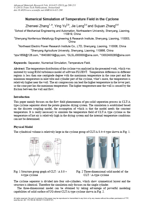
Numerical Simulation of Temperature Field in the CycloneZhenwei Zhang1, a, Ying Yu2,b, Jie Leng3,c and Sujuan Zhang4,d1School of Mechanical Engineering and Automation, Northeastern University, Shenyang, Liaoning,110819, China2Shenyang Nonferrous Metallurgy Engineering & Research Institute, Shenyang, Liaoning, 110003,China3Northeast Electric Power Research Institute Co., LTD, Shenyang, Liaoning, 110006, China 4Shenyang Agriculture University, Shenyang, Liaoning, 110866, Chinaa zzw1658@, b164038019@, c GLSLJ000000@, d130********@ Keywords: Separator, Numerical Simulation, Temperature Field.Abstract. The temperature distribution of the cyclone was analyzed in the presented work, which was imitated by using RSM turbulence model of software FLUENT. Temperature difference in different regions is less than one centigrade degree with the maximum temperature in the cone part and the minimum temperature in inlet tube and cylinder part of the cyclone, what’s more, the temperature is relatively higher near the wall. The air compression can lead the higher temperature in the lower part, so the cone part has the maximum temperature. The higher temperature near the wall is caused by the friction between the wall and flow.IntroductionThis paper mainly focuses on the flow field phenomenon of gas-solid separation process in CLT/A type cyclone separator about the potato granules drying system. The simulation is established based on the discrete coupling model, the assumption of which is that the model needs the constant temperature. It is really necessary to simulate the temperature field of CLT/A type cyclone as the temperature of hot air is relatively high in the drying system and the internal temperature conditions can not be determined.Physical ModelThe cylindrical volume is relatively large in the cyclone group of CLT/A 8.4×4 type shown in Fig. 1. Fig. 1 Structure group graph of CLT / A 8.0 ×4-type cycloneFig. 2 Three-dimensional solid model of theCLT / A-type cycloneThe cyclone separator is divided into four sub-cylinders, which show symmetrical layout and the structure is identical. Therefore the simulation only focuses on the single cylinder.The three-dimensional model can be obtained by taking advantage of powerful modeling capabilities of solid surface of UG about CLT/A type cyclone shown in Fig. 2.Finite Element ModelThe three-dimensional solid model established by UG can be imported into GAMBIT so as to be meshed. Multiple Boolean operations should be carried out on the solid model in order to be facilitated to mesh in GAMBIT, which can lead to the establishment of two entities form. The overall body of Volom1 is consisted of exhaust volute and exhaust pipe. The overall body of Volom2 is consisted of entrance pipe and cone below the cylinder. Then the model will be imported into GAMBIT with the total model shown in Fig. 3. The operations in GAMBIT can be shown as flowing.Fig. 3 Physical model of cyclone in GAMBIT Fig. 4 Mesh diagram of CLT / A-type cyclone(1) Establish the auxiliary plane and split the intake pipe with the Split command.(2) The cylinder can be divided into two parts with a plane parallel to Y-axis at Y=2260mm, the upper of which is ring cylinder with the lower part is cylinder.The entire cyclone is divided into four parts: intake pipe, outtake pipe, lower half part of the cylinder and the upper half part of the cylinder. The meshing can be imposed on them separately. Meshing is the premise process of numerical simulation and also the discrete process of calculating region. The number of the grid has little effect on the simulation result by continuing encryption , when the intensity of the grid reaches a certain value[1]. However, in practice, if the mesh is too sparse, it is so difficult to describe some detail in the flow field, what’s more, the computing speed can be greatly affected if the number of the meshing is too large. Therefore the number select of the grids can both guarantee the accuracy requirements and avoid excessive consumption of the system resources [2]. This paper adopts the complex grids according to the complexity of the flow field and variability of local feature. The hexahedral grid can be generated, which is the main structure, by taking advantage of Hex/Wedge-type structured grid and Cooper barrel pattern. This kind of grid matches well with the flow field, and is conductive to process of coupling conditions in the numerical simulation region. The meshing can be drawn as Fig. 4.Boundary ConditionsThe gas phase can be simplified in order to facilitate solving the multiphase flow inside the cyclone[3].(1) Gas flow is steady-state in cyclone;(2) The gas flow rate is low( generally less than 30m/s), and the gas can be seen as incompressible fluid;(3) The inlet air flows evenly, and in a fully developed turbulent state;(4) No gas exhausts from the dust exhaust at the bottom of the cyclone.Boundary conditions set as following:(1) Inlet boundary: the inlet air temperature is 373.3K, and the density is 1.225Kg/m3. The viscosity is 18.1×10⁻⁶ . Assuming that the inlet turbulent is developed fully, and the gas inlet velocity is set as 15m/s evenly distribution throughout the inlet section. The turbulence intensity is set as I and the hydraulic diameter is set as D. Flow Reynolds number is shown as Eq. 1.4e 61.225150.252R 2.5725101810UD ρµ−××===×× (1)Hydraulic diameter is set as Eq. 2.220.460.2070.2940.460.207HD ab D a b ××===++ (2) Turbulence Intensity is set as Eq. 3.1/851/8e 0.16(R )100%0.16(2.5710)7.34%I −−=×=××= (3)(2) Outlet boundary: outlet boundary is set as outflow boundary. Assuming that the flow condition is in fully developed condition, namely the flow situation can be obtained by the pulling of flow field. The air exhaust can be set as the outflow, and the weight of the flow is set as one. The dust exhaust is set as outflow, and the weight of the flow is set as zero.(3) Wall conditions: take the standard wall function, namely the wall has no-slip boundary [4]. The roughness parameter of wall is set as 0.5.(4) The overlapping circle is set as interface surface, which connects the exhaust pipe and cylinder. Numerical Simulation AnalysisTemperature distribution at various locations in CLT/A type cyclone can be intuitively obtained through numerical simulation shown in the Fig. 5. The entrance temperature is relatively low, and temperature can increase with moving downward along the cone. The value can reach the highest at the bottom of cone. The exhaust temperature can decrease along the exhaust pipe, but is still higher than inlet air temperature. The temperature change reason is shown as following: the air enters the air intake with the number of 100, and the flow can be compressed by centrifugal force caused by the rotation. In addition, the temperature can be increased due to the friction between the flow and wall. The temperature continues to rise owing to the further impact of compression and friction when reaches the cone wall.Fig. 6 and Fig. 7 respectively show the temperature distribution in Y=0 section about moderate and total temperature in CLT/A type cyclone separator. The moderate temperature distribution has the same situation with the total temperature distribution in the Y=0 cross section in the cyclone. The temperature of air intake and cylinder is the lowest with the maximum temperature in the cone part, and the temperature of exhaust pipe stays centre. The exhaust pipe temperature can decrease further. Temperature distribution shows a symmetrical situation in both sides of the exhaust pipe or inside it in cyclone with only little difference near the wall, which shows the vortex shape. The small difference is caused by the local turbulence accompanied by the rotation flow inside cyclone.Fig. 5 Total temperature field Fig. 6 Y=0 Static temperature Fig. 7 Y=0 Total temperature Fig. 8 and Fig. 9 respectively show the temperature distribution in X=0 section about static and total temperature in CLT/A type cyclone separator. Internal temperature distribution of X=0 section has the same situation with the total temperature distribution in cyclone. The cylinder part below the exhaust pipe has almost the same temperature distribution with the lower cone compared with the section Y=0 with only obvious difference in the position above the air exhaust, the reason for which is that the asymmetry caused the flow’s entrance from the unilateral line.Fig. 8 X=0 Static temperature Fig. 9 X=0 Total temperatureFig. 10 The temperature distribution on Z = 0.5, 0.75, 1, 1.25, 1.5, 1.75, 2 cross section Fig. 10 shows that temperature near the wall is relatively high, the reason for which is that friction between the flow and wall and compression effect of centrifugal force can lead the enhancement of temperature. Temperature gradient of each cross-section shows circular ring, better symmetry and a certain degree irregularity that can be caused by the different local turbulence.ConclusionThis thesis puts forward the temperature distribution of the cyclone with type of CLT/A, and figures out that the overall temperature is about 373°C. Temperature difference in different region is less than one centigrade degree with the maximum temperature in the cone part and the minimum temperature in inlet tube and cylinder part of the cyclone, what’s more, the temperature is relatively higher near the wall. The air compression can lead the higher temperature in the lower part, so the cone part has the maximum temperature which is caused by the strengthen impact of air compression. The higher temperature near the wall is caused by the friction between the wall and flow. The total temperature in the cyclone stays a constant value with almost no change and local difference can be obtained. Reference[1] F. Boysan, J. Ewan and B. Swithen. Experimental and Theoretical Studies of Cyclone SeparatorAerodynamics: (Chem E Symp Series, PP. 305-320, 1983).[2] W. Q. Tao. Modern Process of Heat Transfer Calculation: (Science Press, 2002).[3] G. L. Gao. Thermal Engineering and Fluid Mechanics: (China Electric Power Press, PP. 130-131, China 1997).[4] Y. Mao, L. Pang, X. W. Wang et al. Numerical Simulation of Three-dimensional Turbulence inCyclone: (Petroleum Refining and Chemical Industry, V. 33(2), PP. 1-6, China 2002).。


Title: Numerical Simulation of Welding for Composite Aluminum-copper Foils1. IntroductionIn recent years, the demand for high-performance petposite materials has been increasing, with aluminum-copper foils being one of the mostmonly used materials for this purpose. The welding of theseposite foils plays a crucial role in determining the overall performance of the final product. In order to optimize the welding process, numerical simulation has been widely used to study the heat transfer, material flow, and microstructure evolution during the welding process. In this article, we will discuss the latest developments in the numerical simulation of welding forposite aluminum-copper foils.2. Material Properties2.1 Aluminum-copper FoilsAluminum-copper foils areposite materials consisting of layers of aluminum and copper. The different coefficients of thermal conductivity and melting points of aluminum and copper make the welding process more challengingpared to conventional foil materials.2.2 Welding ParametersThe welding parameters, including welding speed, heat input, and pressure, have a significant impact on the quality of the welded joint. The optimization of these parameters is crucial for achieving a high-quality weld.3. Numerical Simulation Methods3.1 Finite Element Method (FEM)FEM is a widely used numerical simulation method for studying the welding process. It can simulate the heat transfer, material flow, and stress distribution during welding, providing valuable insights into the welding process.3.2 Computational Fluid Dynamics (CFD)CFD is another powerful tool for simulating the fluid flow and heat transfer during the welding process. It can help optimize the welding process by predicting the flow patterns and temperature distribution in the weld pool.4. Modeling of Welding Process4.1 Heat TransferThe heat transfer in the welding process is a critical factor affecting the temperature distribution in the weld pool.Numerical simulation can predict the temperature field and thermal history of the welded joint, providing guidance for optimizing the welding process.4.2 Material FlowThe material flow in the weld pool determines the microstructure and mechanical properties of the welded joint. Numerical simulation can predict the flow patterns and solidification behavior, 本人ding in the design of a high-quality weld.5. Microstructure EvolutionThe microstructure evolution during the welding process plays a crucial role in determining the mechanical properties of the welded joint. Numerical simulation can predict the gr本人n growth and phase transformation, providing valuable information for optimizing the welding parameters.6. Validation of Numerical SimulationExperimental validation of the numerical simulation results is essential to ensure the accuracy and reliability of the simulation. In-situ observations and mechanical testing can validate the microstructure and mechanical properties of the welded joint.7. Applications and Future DevelopmentsNumerical simulation of welding forposite aluminum-copper foils has been widely used in the pet industry to optimize the welding process and improve the quality of the welded joints. In the future, further developments in numerical simulation methods and material characterization techniques will continue to advance the understanding and optimization of the welding process forposite pet materials.8. ConclusionIn conclusion, numerical simulation plays a crucial role in the study and optimization of the welding process forposite aluminum-copper foils. By simulating the heat transfer, material flow, and microstructure evolution, numerical simulation provides valuable insights into the welding process, enabling the design of high-quality welded joints. With further advancements in numerical simulation methods and material characterization techniques, the welding ofposite pet materials will continue to improve, meeting the increasing demand for high-performance pet products.。
浮法玻璃锡槽内保护气体流动状态的三维数值模拟闫亚琼续芯如徐洋冯建业贾立丹陈福(秦皇岛玻璃工业研究设计院有限公司秦皇岛市 066004)摘要在分析浮法玻璃锡槽结构的基础上,建立了浮法玻璃锡槽的三维物理模型,利用有限元模拟主要研究了在玻璃锡槽中随着气体不断地从进气口喷人,保护气体(n2+h2)的体积分数分布及速度场变化情况。
关键词锡槽保护气体数值模拟体积分数速度场中图分类号:TQ171 文献标识码:A文章编号:1003-1987(2018)09-0005-04Three Dimensional Numerical Simulationof the Protective Gas Flow in a Tin Bath ofFloat ProcessYAN Yaqiong,X U X in ru,XU Yang,FENGJianye,JIA Lidan,CHENFu (Qinhuangdao Glass Industry Research and design Institute Company Limited,Qinhuangdao,066004 ) Abstract: Based on the analysis on the structure o f tin bath,the mathematical model in a tin bath o f floating glass is established.As the protective gas continues to flow from the air in le t,the distribution o f volume fraction and velocity field o f protective gases(nitrogen and hydrogen)is m ainly studied by using the method o f finite element modeling.Key Words: tin bath,protective gas,numerical simulation,volume fraction,velocity field〇引言锡槽是浮法玻璃生产过程中的重要热工设 备,是玻璃成型区。
a rXiv:as tr o-ph/69732v127Se p26Simulation of the Magnetothermal Instability Ian J.Parrish and James M.Stone 1Department of Astrophysical Sciences,Princeton University,Princeton,NJ 08544ABSTRACT In many magnetized,dilute astrophysical plasmas,thermal conduction occurs almost exclusively parallel to magnetic field lines.In this case,the usual stability criterion for convective stability,the Schwarzschild criterion,which depends on entropy gradients,is modified.In the magnetized long mean free path regime,instability occurs for small wavenumbers when (∂P/∂z )(∂ln T/∂z )>0,which we refer to as the Balbus criterion.We refer to the convective-type instability that results as the magnetothermal instability (MTI).We use the equations of MHD with anisotropic electron heat conduction to numerically simulate the linear growth and nonlinear saturation of the MTI in plane-parallel atmospheres that are unstable according to the Balbus criterion.The linear growth rates measured from the simulations are in excellent agreement with the weak field dispersion relation.The addition of isotropic conduction,e.g.radiation,or strong magnetic fields can damp the growth of the MTI and affect the nonlinear regime.The instability saturates when the atmosphere becomes isothermal as the source of free energy is exhausted.By maintaining a fixed temperature difference between the top and bottom boundaries of the simulation domain,sustained convective turbulence can be driven.MTI-stable layers introduced by isotropic conduction are used to prevent the formation of unresolved,thermal boundary layers.Wefind that the largest component of the time-averaged heat flux is due to advective motions as opposed to the actual thermal conduction itself.Finally,we explore the implications of this instability for a variety of astrophysical systems,such as neutron stars,the hot intracluster medium of galaxy clusters,and the structure of radiatively inefficient accretion flows.Subject headings:accretion,accretion disks —convection —hydrodynamics —instabilities —MHD —stars:neutron —turbulence1.IntroductionIn many dilute,magnetized astrophysical plasmas,the electron mean free path between collisions can be many orders of magnitude larger than the ion gyroradius.In this regime, the equations of ideal magnetohydrodynamics(MHD)that describe thefluid plasma must be supplemented with anisotropic transport terms for energy and momentum due to the near free-streaming motions of particles along magneticfield lines(Braginskii1965).Thermal conduction is dominated by the electrons compared to ions by a factor of the square root of the mass ratio.In a non-rotating system,it is sufficient to neglect the ion viscosity(Balbus 2004).A fully collisionless treatment may be done using more complex closures such as Hammett&Perkins(1990).The implications of anisotropic transport terms on the overall dynamics of dilute as-trophysical plasmas is only beginning to be explored(Balbus2001;Quataert,Hammett,& Dorland2002;Sharma,Hammett,&Quataert2003).One of the most remarkable results obtained thus far is that the convective stability criterion for a weakly magnetized dilute plasma in which anisotropic electron heat conduction occurs is drastically modified from the usual Schwarzschild criteria(Balbus2000).In particular,stratified atmospheres are unstable if they contain a temperature(as opposed to entropy)profile which is decreasing upward.There are intriguing analogies between the stability properties of rotationally sup-portedflows(where a weak magneticfield changes the stability criterion from a gradient of specific entropy to a gradient of angular velocity),and the convective stability of stratified atmospheres(where a weak magneticfield changes the stability criterion from a gradient of entropy to a gradient of temperature).The former is a result of the magnetorotational instability(MRI;Balbus&Hawley1998).The latter is a result of anisotropic heat con-duction.To emphasize the analogy,we will refer to this new form of convective instability as the magnetothermal instability(MTI).The MTI may have profound implications for the structure and dynamics of many astrophysical systems.In this paper,we use numerical methods to explore the nonlinear evolution and satu-ration of the MTI in two-dimensions.We adopt an arbitrary vertical profile for a stratified atmosphere in which the entropy increases upward(and therefore is stable according to the Schwarzschild criterion),but in which the temperature is decreasing upwards(and there-fore is unstable according to the Balbus criterion,(∂P/∂z)(∂ln T/∂z)<0).We confirm the linear growth rates predicted by Balbus(2000)for dynamically weak magneticfields and numerically measure the growth rates for strongerfields.Wefind that in the nonlinear regime vigorous convective turbulence results in efficient heat transport.Full details are published in Parrish&Stone(2005),hereafter PS.These results may have implications for stratified atmospheres where anisotropic trans-port may be present.The most exciting potential application is to the hot X–ray emitting gas in the intracluster medium of galaxy clusters(Peterson&Fabian2005;Markevitch 1998).The hot plasmas are magnetized and have very long mean free paths along the mag-neticfield lines;thus,they are a prime candidate for this instability.For example,the Hydra A cluster has T≈4.5keV and a density of n≈10−3−10−4cm−3giving a mean free path that’s almost one-tenth of the virial radius.Other applications are to the atmospheres of neutron stars with moderate magneticfields and radiatively inefficient accretionflows.2.Physics of the MTI2.1.Equations of MHD and Linear StabilityThe physics of the MTI is described by the usual equations of ideal MHD with the addition of a heatflux,Q,and a vertical gravitational acceleration,g.∂ρ∂t+∇· ρvv+ p+B24π +ρg=0,(2)∂B∂t+∇· v E+p+B24π +∇·Q+ρg·v=0,(4) where the symbols have their usual meaning with E the total energy.The heatflux contains contributions from electron motions(which are constrained to move primarily alongfield lines)and isotropic transport,typically due to radiative processes.Thus,Q=Q C+Q R, whereQ C=−χCˆbˆb·∇T,(5)Q R=−χR∇T,(6) whereχC is the Spitzer Coulombic conductivity(Spitzer1962),ˆb is a unit vector in the direction of the magneticfield,andχR is the coefficient of isotropic conductivity.Some progress can be made analytically in the linear regime of the instability.I introduce two useful quantities,χ′C=γ−1P(χC+χR).(7)With WKB theory,one is able to obtain a dispersion relation.The details of this process are to be found in§4of Balbus(2000).The most important result of the linear analysis isthe instability criterion,k2v2A−χ′C∂z∂ln T∂z∂ln Td ln R>0,(10) whereΩis the angular velocity.The similarity between the MRI and the MTI is self-evident.Strong magneticfields are capable of stabilizing short-wavelenth perturbations in both instabilities through magnetic tension.putational MethodWe use the3D MHD code ATHENA(Gardiner&Stone2005)with the addition of an operator-split anisotropic thermal conduction module for our simulations.Our initial state is always a convectively stable state(dS/dz>0)in hydrodynamic equilibrium.We implement two different boundary conditions for exploring the nonlinear regime.Thefirst boundary condition is that of an adiabatic boundary condition at the upper and lower boundaries,i.e.a Neumann boundary condition on temperature.This situation is ideal for single-mode studies of linear growth rates.In the Neumann boundary condition the magneticfield is reflected at the upper and lower boundaries,consistent with the adiabatic condition on heatflow.The second boundary conditionfixes the the temperature at the upper and lower boundaries of the atmosphere,i.e.a Dirichlet boundary condition on temperature.This setup is useful for driven simulations where we wish to study the effects of turbulence.In this boundary condition,the magneticfield is again reflected at the boundaries of the box,but heat is permitted toflow across the boundary from the constant temperature ghost zones.With these choices of boundary conditions,the net magneticflux penetrating the box is constant in time as there is zero Maxwell stress at the boundary.If the net magneticflux penetrating the box is initially zero,then in two dimensions the magnitude of the magneticfield mustdecay in time as a result of Cowling’s anti-dynamo theorem,but otherwise the saturated state is not affected.3.Results3.1.Single-Mode Perturbation and Qualitative Understanding of the MTIBy examining a single mode-perturbation to the background state,we can gain an intuitive understanding of the physical mechanism of the instability.We begin by perturbing a convectively-stable,but MTI-unstable atmosphere with a very weak sub-sonic and sub-Alf´e nic sinusoidal velocity perturbation in a box with adiabatic boundary conditions.The evolution of the magneticfield lines is shown in Figure1for several different times.Notice in the upper right plot that at x≈0.03that a parcel offluid(as traced by the frozen-in field line)has been displaced upward in the atmosphere.As this parcel offluid comes to mechanical equilibirum with the background state,it adiabatically cools.The magnetic field line now is partially aligned with the background temperature state,thus thermally connecting this parcel offluid with a hotter parcel deeper in the atmosphere.As a result, heatflows along thefield,causing the higher parcel to become buoyant.This buoyant motion causes thefield line to be more aligned with the background temperature,increasing the heat flux,and generating a runaway instability.It is instructive to examine the behavior of the temperature profile of the atmosphere. Figure2shows the horizontally averaged temperature profile of this run at various times (normalized to the sound crossing time).The initial state is a linear temperature profile decreasing with height.As the instability progresses,the temperature profile becomes more and more isothermal.Saturation occurs,as one would expect,when the temperature profile is almost completely isothermal,since the source of free energy has been depleted.More details are to be found in§4of PS.3.2.Linear Growth RatesBy following§4.3of Balbus(2000)and using the Fourier convention,exp(σt+ikx), one can derive a weak-field dispersion relation for the MTI asσγ σN + σd ln S χ′c T k2where N is the Brunt-V¨a is¨a l¨a frequency,the natural frequency of adiabatic oscillations for an atmosphere.With the single-mode perturbation simulations we are able to measure the growth rate for a variety of situations.Figure3plots the nondimensionalized growth rate versus wavenumber for theory(solid line)and the measured values from simulations(crosses). As can be seen these are in very good agreement.There are essentially two ways to suppress the growth of the MTI.First,strong magnetic fields can exert tension that limits the growth and saturation of the instability.Second, isotropic conduction,as would result from radiative transport,can effectively short-circuit the thermal driving alongfield lines necessary for this instability to occur.For more detailed analysis,we refer the reader to§3of PS.3.3.Nonlinear Regime and Efficiency of Heat TransportIn order to assess the efficiency of heat transport in the magnetothermal instability,one needs to examine multimode simulations seeded with Gaussian white noise perturbations and conducting boundary conditions at the top and bottom of the domain.The simplest such set-up results in narrow,unresolved boundary layers at the upper and lower boundaries, thus,making the heatflux difficult to measure accurately.As an alternative,we utilize a more physically relevant simulation.This setup involves an atmosphere that is convectively stable throughout,but MTI unstable only in the central region.The surrounding regions are stabilized to the MTI through the addition of isotropic conducitivity.As a result,the central unstable region is well-resolved.Figure4shows the evolution of magneticfield lines as this instability progresses.The magneticfield lines shown essentially track the central unstable region;however,the third panel clearly shows a plume offluid that is penetrating into the stable layer as a result of convective overshoot.This phenomenon is well-known in the solar magnetoconvection literature(Tobias,et al.2001;Brummell,Clune,&Toomre 2002).In three dimensions this type of behavior greatly amplifies the magneticfield in a local magnetic dynamo.More quantitative measurements can be made by comparing the time-and horizontally-averaged vertical heatfluxes and breaking it down into Coulombic,radiative,and isotropic components.Figure5shows these quantities plotted as a function of time.At the mid-plane,the oscillatory advectiveflux is clearly dominant at any given instant in time;how-ever,averaged in time the advective heatflux contributes roughly2.3 To determine the heat conduction efficiency of this instability,we compare it to the ex-pected vertical heatflux across the simulation domain for pure uniform isotropic conduc-tivity,namely,Q0≈3.33×10⁻⁵.The time-averaged heat conduction at the midplane is Q tot,50% ≈3.54×10⁻⁵,which indicates that the instability transports the entire applied heatflux efficiently.4.Conclusions and ApplicationThe most important conclusion of this work is that atmospheres with dS/dZ<0are not necessarily stable to convection.In fact,dilute atmospheres with weak to moderate magnetic fields can be convectively unstable by the Balbus criterion resulting in an instability that we call the magnetothermal instability.We have verified using MHD simulations that the measured linear growth rates agree with analytic WKB theory as predicted by Balbus(2000). For adiabatic boundary conditions,wefind the saturated state is an isothermal temperature profile,corresponding to the exhaustion of the free energy in the system.For a driven instability with conducting boundary conditions,wefind that the MTI efficiently transports heat,primarily by advective motions of the plasma in the vigorous convection that results.The most promising application of this instability is to clusters of galaxies.Structure formation calculations assumingΛCDM cosmologies predict monotonically decreasing tem-perature profiles of the intracluster gas(Loken,et al2002).Observations of clusters with Chandra,such as Hydra A(DeGrandi&Modlendi2002),however,indicate essentiallyflat temperature profiles.The intracluster medium is dilute,magnetized,and has a mean free path that could be as high as one-tenth of the cluster virial radius.It may be that these temperature profiles are representative of the saturated state of the MTI.This possibility will be explored in future work.REFERENCESBalbus,S.A.,&Hawley J.F.1998,Rev.Mod.Phys.,70,1Balbus,S.A.2000,ApJ,534,420Balbus,S.A.2001,ApJ,562,909Balbus,S.A.2004,ApJ,616,857Braginskii,S.I.1965,in Reviews of Plasma Physics,Vol.1,ed.M.A.Leontovich(New York:Consultants Bureau),205Brummell,N.H.,Clune,&T.L.,Toomre,J.2002,ApJ,570,825DeGrandi,S.,&Molendi,S.2002,ApJ,567,163Gardiner,T.&Stone,J.2005,p.Phys.,205,509 Hammett,G.W.&Perkins,F.W.1990,Phys.Rev.Lett.,64,3019 Loken,C.,et al2002,ApJ,579,571Markevitch,M.,et al.1998,ApJ,377,392Parrish,I.J.,&Stone,J.M.,ApJ633,334Peterson,J.R.,&Fabian,A.C.2005,astro-ph0512549 Quataert,E.,Dorland,W.,&Hammett,G.W.2002ApJ,577,524 Sharma,P.,Hammett,G.,Quataert,E.2003,ApJ,596,1121 Spitzer,L.1962,Physics of Fully Ionized Gases(New York:Wiley) Tobias,S.M.,et al.2001,ApJ,549,1183Fig.1.—Snapshots of the magneticfield lines for a single-mode perturbation with adiabatic boundary conditions at various times during the evolution of the instability.(upper left) Inititial condition;(upper right)Linear phase;(lower left)Non-linear phase;(lower right) Saturated state.Fig.2.—Vertical profile of the horizontally-averaged temperature profile in the single mode case at various times.The initial state is a monotonically decreasing temperature profilewith respect to height,and thefinal state is isothermal.Fig.3.—Solutions of the MTI dispersion relation in the weakfield limit for an atmosphere with d ln T/d ln S=−3.The axes are normalized to the local Brunt-V¨a is¨a l¨a frequency,N. The crosses are growth rates measured from simulations.Fig.4.—Snapshots of the magneticfield in the run with stable layers.(far left)Early linear phase;(middle left)early non-linear phase.(middle right)The MTI drives penetrative convection into the stable layers,and at late times(far right)magneticflux is pumped into the stable layers.Fig. 5.—Time evolution of the horizontally-averaged heatflux at the midplane and80% height of the simulation domain in the run with stable layers.The total heatflux(thick solid line)is subdivided into Coulombic(thin solid line),radiative(dashed lined),and advective (dotted line)components.The instantaneous total heatflux is dominated by advective motions.。