计量经济学导论第四版第一章
- 格式:pptx
- 大小:781.54 KB
- 文档页数:26


第一章 绪论1.1 一般说来,计量经济分析按照以下步骤进行:(1)陈述理论(或假说) (2)建立计量经济模型 (3)收集数据(4)估计参数 (5)假设检验 (6)预测和政策分析 1.2 我们在计量经济模型中列出了影响因变量的解释变量,但它(它们)仅是影响因变量的主要因素,还有很多对因变量有影响的因素,它们相对而言不那么重要,因而未被包括在模型中。
为了使模型更现实,我们有必要在模型中引进扰动项u 来代表所有影响因变量的其它因素,这些因素包括相对而言不重要因而未被引入模型的变量,以及纯粹的随机因素。
1.3时间序列数据是按时间周期(即按固定的时间间隔)收集的数据,如年度或季度的国民生产总值、就业、货币供给、财政赤字或某人一生中每年的收入都是时间序列的例子。
横截面数据是在同一时点收集的不同个体(如个人、公司、国家等)的数据。
如人口普查数据、世界各国2000年国民生产总值、全班学生计量经济学成绩等都是横截面数据的例子。
1.4 估计量是指一个公式或方法,它告诉人们怎样用手中样本所提供的信息去估计总体参数。
在一项应用中,依据估计量算出的一个具体的数值,称为估计值。
如Y 就是一个估计量,1nii YY n==∑。
现有一样本,共4个数,100,104,96,130,则根据这个样本的数据运用均值估计量得出的均值估计值为5.107413096104100=+++。
第二章 计量经济分析的统计学基础2.1 略,参考教材。
2.2N SS x ==45=1.25 用α=0.05,N-1=15个自由度查表得005.0t =2.947,故99%置信限为x S t X 005.0± =174±2.947×1.25=174±3.684也就是说,根据样本,我们有99%的把握说,北京男高中生的平均身高在170.316至177.684厘米之间。
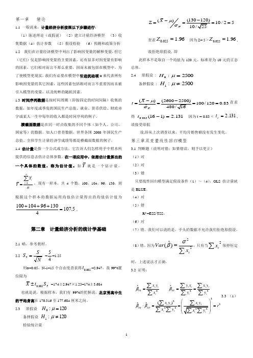
2.3 原假设120:0=μH备择假设120:1≠μH检验统计量()10/25XX μσ-Z ====查表96.1025.0=Z 因为Z= 5 >96.1025.0=Z ,故拒绝原假设, 即此样本不是取自一个均值为120元、标准差为10元的正态总体。


伍德里奇计量经济学导论第4版视频精讲!伍德里奇《计量经济学导论》(第4版)精讲班【教材精讲+考研真题串讲】来源:攻关学习网讲师:张冠甲/闫晶晶目录说明:本课程共包括42个高清视频(共54课时)。
序号名称1绪论2第1章计量经济学的性质与经济数据3第2章简单回归模型(1)4第2章简单回归模型(2)5第3章多元回归分析:估计(1)6第3章多元回归分析:估计(2)7第3章多元回归分析:估计(3)8第4章多元回归分析:推断(1)9第4章多元回归分析:推断(2)10第4章多元回归分析:推断(3)11第5章多元回归分析:OLS的渐进性(1)12第5章多元回归分析:OLS的渐进性(2)13第6章多元回归分析:深入专题(1)14第6章多元回归分析:深入专题(2)15第7章含有定性信息的多元回归分析:二值(或虚拟)变量(1)16第7章含有定性信息的多元回归分析:二值(或虚拟)变量(2)17第8章异方差性(1)18第8章异方差性(2)19第8章异方差性(3)20第8章异方差性(4)21第8章异方差性(5)22第9章模型设定和数据问题的深入探讨(1)23第9章模型设定和数据问题的深入探讨(2)24第9章模型设定和数据问题的深入探讨(3)25第9章模型设定和数据问题的深入探讨(4)26第9章模型设定和数据问题的深入探讨(5)27第10章时间序列数据的基本回归分析(1)28第10章时间序列数据的基本回归分析(2)29第11章OLS用于时间序列数据的其他问题(1)30第11章OLS用于时间序列数据的其他问题(2)31第12章时间序列回归中的序列相关和异方差(1)32第12章时间序列回归中的序列相关和异方差(2)33第13章跨时横截面的混合:简单面板数据方法(1)34第13章跨时横截面的混合:简单面板数据方法(2)35第14章高深的面板数据方法(1)36第14章高深的面板数据方法(2)37第15章工具变量估计与两阶段最小二乘法(1)38第15章工具变量估计与两阶段最小二乘法(2)39第16章联立方程模型40第17章限值因变量模型和样本选择纠正01:31:3241第18章时间序列高级专题42第19章一个经验项目的实施内容简介本课程是伍德里奇《计量经济学导论》(第4版)网授精讲班,为了帮助参加研究生招生考试指定考研参考书目为伍德里奇《计量经济学导论》(第4版)的考生复习专业课,我们根据教材和名校考研真题的命题规律精心讲解教材章节内容。
第1章 导论一、选择题1.在计量经济模型中,入选的每一个解释变量之间都是( )。
A.函数关系B.非线性相关关系C.简单相关关系D.独立的【答案】D【解析】计量经济学模型的所有解释变量共同对被解释变量起到解释作用,所有的解释变量之间应为相互独立的。
若解释变量之间存在相关关系,这将会导致模型出现多重共线性问题,参数估计将会出现偏误。
2.下列各项中,属于截面数据的是( )。
A.1990~2018年我国居民的收入B.1990~2018我国的出口额C.2018年第一季度15个重点调查的煤炭行业各种产品的产量D.2018年第一季度15个重点调查的煤炭企业的产量【答案】D【解析】截面数据是一批发生在同一时间截面上的调查数据,用截面数据作为计量经济学模型的样本数据,需要注意两个问题:①样本与母体的一致性问题。
截面数据很难用于一些总量模型的估计;②模型随机干扰项的异方差问题。
AB两项是时间序列数据;C项3.对模型中参数估计量的符号、大小、相互之间的关系进行检验,属于( )。
A.经济意义检验B.计量经济学检验C.统计检验D.稳定性检验【答案】A【解析】经济意义检验主要检验模型参数估计量在经济意义上的合理性,主要方法是将模型参数的估计量与预先拟定的理论期望值进行比较,包括参数估计量的符号、大小、相互之间的关系;计量经济学检验主要检验模型的计量经济学性质,主要有自相关检验、异方差检验、多重共线性检验等;统计检验主要检验模型参数估计值的可靠性,主要有F 检验、t检验、拟合优度检验等;稳定性检验主要检验模型参数的稳定性,主要方法包括Chow检验、LR检验、随机系数法等。
二、判断题1.计量经济学是一门应用数学学科。
( )【答案】×【解析】计量经济学是经济学的一个分支学科,即它是一门经济学科,而不是应用数学或其他学科。
2.人口普查数据属于时间序列数据。
( )【解析】时间序列数据是一个或多个变量按照时间先后排列的统计数据,而“人口普查数据”是一个或多个变量发生在同一时间截面上的调查数据,即属于截面数据。
236APPENDIX BSOLUTIONS TO PROBLEMSB.1 Before the student takes the SAT exam, we do not know – nor can we predict with certainty – what the score will be. The actual score depends on numerous factors, many of which we cannot even list, let alone know ahead of time. (The student’s innate ability, how the student feels on exam day, and which particular questions were asked, are just a few.) The eventual SAT score clearly satisfies the requirements of a random variable.B.2 (i) P(X ≤ 6) = P[(X – 5)/2 ≤ (6 – 5)/2] = P(Z ≤ .5) ≈ .692, where Z denotes a Normal (0,1) random variable. [We obtain P(Z ≤ .5) from Table G.1.](ii) P(X > 4) = P[(X – 5)/2 > (4 – 5)/2] = P(Z > −.5) = P(Z ≤ .5) ≈ .692.(iii) P(|X – 5| > 1) = P(X – 5 > 1) + P(X – 5 < –1) = P(X > 6) + P(X < 4) ≈ (1 – .692) + (1 – .692) = .616, where we have used answers from parts (i) and (ii).B.3 (i) Let Y it be the binary variable equal to one if fund i outperforms the market in year t . By assumption, P(Y it = 1) = .5 (a 50-50 chance of outperforming the market for each fund in each year). Now, for any fund, we are also assuming that performance relative to the market is independent across years. But then the probability that fund i outperforms the market in all 10 years, P(Y i 1 = 1,Y i 2 = 1, …, Y i ,10 = 1), is just the product of the probabilities: P(Y i 1 = 1)⋅P(Y i2 =1) … P(Y i ,10 = 1) = (.5)10 = 1/1024 (which is slightly less than .001). In fact, if we define a binary random variable Y i such that Y i = 1 if and only if fund i outperformed the market in all 10 years, then P(Y i = 1) = 1/1024.(ii) Let X denote the number of funds out of 4,170 that outperform the market in all 10 years. Then X = Y 1 + Y 2 + … + Y 4,170. If we assume that performance relative to the market is independent across funds, then X has the Binomial (n ,θ) distribution with n = 4,170 and θ = 1/1024. We want to compute P(X ≥ 1) = 1 – P(X = 0) = 1 – P(Y 1 = 0, Y 2 = 0, …, Y 4,170 = 0) = 1 – P(Y 1 = 0)⋅ P(Y 2 = 0)⋅⋅⋅P(Y 4,170 = 0) = 1 – (1023/1024)4170 ≈ .983. This means, if performance relative to the market is random and independent across funds, it is almost certain that at least one fund will outperform the market in all 10 years.(iii) Using the Stata command Binomial(4170,5,1/1024), the answer is about .385. So there is a nontrivial chance that at least five funds will outperform the market in all 10 years.B.4 We want P(X ≥.6). Because X is continuous, this is the same as P(X > .6) = 1 – P(X ≤ .6) = F (.6) = 3(.6)2 – 2(.6)3 = .648. One way to interpret this is that almost 65% of all counties have an elderly employment rate of .6 or higher.B.5 (i) As stated in the hint, if X is the number of jurors convinced of Simpson’s innocence, then X ~ Binomial(12,.20). We want P(X ≥ 1) = 1 – P(X = 0) = 1 – (.8)12 ≈ .931.课后答案网 w w w .k h d a w .c o m237(ii) Above, we computed P(X = 0) as about .069. We need P(X = 1), which we obtain from(B.14) with n = 12, θ = .2, and x = 1: P(X = 1) = 12⋅ (.2)(.8)11 ≈ .206. Therefore, P(X ≥ 2) ≈ 1 – (.069 + .206) = .725, so there is almost a three in four chance that the jury had at least two members convinced of Simpson’s innocence prior to the trial.B.6 E(X ) = 30()xf x dx ∫ = 320[(1/9)] x x dx ∫ = (1/9) 330x dx ∫. But 330x dx ∫ = (1/4)x 430| = 81/4. Therefore, E(X ) = (1/9)(81/4) = 9/4, or 2.25 years. B.7 In eight attempts the expected number of free throws is 8(.74) = 5.92, or about six free throws. B.8 The weights for the two-, three-, and four-credit courses are 2/9, 3/9, and 4/9, respectively. Let Y j be the grade in the j th course, j = 1, 2, and 3, and let X be the overall grade point average. Then X = (2/9)Y 1 + (3/9)Y 2 + (4/9)Y 3 and the expected value is E(X ) = (2/9)E(Y 1) + (3/9)E(Y 2) + (4/9)E(Y 3) = (2/9)(3.5) + (3/9)(3.0) + (4/9)(3.0) = (7 + 9 + 12)/9 ≈ 3.11. B.9 If Y is salary in dollars then Y = 1000⋅X , and so the expected value of Y is 1,000 times the expected value of X , and the standard deviation of Y is 1,000 times the standard deviation of X . Therefore, the expected value and standard deviation of salary, measured in dollars, are $52,300 and $14,600, respectively. B.10 (i) E(GPA |SAT = 800) = .70 + .002(800) = 2.3. Similarly, E(GPA |SAT = 1,400) = .70 + .002(1400) = 3.5. The difference in expected GPAs is substantial, but the difference in SAT scores is also rather large. (ii) Following the hint, we use the law of iterated expectations. Since E(GPA |SAT ) = .70 + .002 SAT , the (unconditional) expected value of GPA is .70 + .002 E(SAT ) = .70 + .002(1100) = 2.9. 课后答案网 w w w .k h d a w .c o m。