第1章 Introductory Econometrics for Finance(金融计量经济学导论-东北财经大学 陈磊)

《金融时间序列分析》讲义主讲教师：徐占东登录：徐占东《金融时间序列模型》参考教材：1．《金融时间序列的经济计量学模型》经济科学出版社米尔斯著2．《经济计量学手册》章节3．《Introductory Econometrics for Finance》 Chris Brooks 剑桥大学出版社4．《金融计量学：资产定价实证分析》周国富著北京大学出版社5．《金融市场的经济计量学》 Andrew lo等上海财经大学出版社6．《动态经济计量学》 Hendry著上海人民出版社7．《商业和经济预测中的时间序列模型》中国人民大学出版社弗朗西斯著8．《No Linear Econometric Modeling in Time series Analysis》剑桥大学出版社9．《时间序列分析》汉密尔顿中国社会科学出版社10．《高等时间序列经济计量学》陆懋祖上海人民出版社11．《计量经济分析》张晓峒经济科学出版社12．《经济周期的波动与预测方法》董文泉高铁梅著吉林大学出版社13．《宏观计量的若干前言理论与应用》王少平著南开大学出版社14．《协整理论与波动模型——金融时间序列分析与应用》张世英、樊智著清华大学出版社15．《协整理论与应用》马薇著南开大学出版社16．（NBER working paper）17．（Journal of Finance）18．（中国金融学术研究网） 教学目的：1）能够掌握时间序列分析的基本方法；2）能够应用时间序列方法解决问题。

教学安排1单变量线性随机模型：ARMA ; ARIMA; 单位根检验。

2单变量非线性随机模型：ARCH,GARCH系列模型。

3谱分析方法。

4混沌模型。

5多变量经济计量分析：V AR模型，协整过程；误差修正模型。

第一章引论第一节金融学简介一．金融学概论1．金融学：研究人们在不确定环境中进行资源最优配置的学科。

金融学的三个核心问题：资产时间价值，资产定价理论（资源配置系统）和风险管理理论。

第1篇横截面数据的回归分析
第1章计量经济学的性质与经济数据
1.1 什么是计量经济学?
1.2 经验经济分析的步骤
1.3 经济数据的结构
1.4 计量经济分析中的因果关系和其他条件不变的概念
小结
关键术语
习题
计算机习题
第2章简单回归模型
第3章多元回归分析：估计
第4章多元回归分析：推断
第5章多元回归分析：OLS的渐近性
第6章多元回归分析：深入专题
第7章含有定性信息的多元回归分析：二值(或虚拟)变量第8章异方差性
第9章模型设定和数据问题的深入探讨
第2篇时间序列数据的回归分析
第10章时间序列数据的基本回归分析
第11章OLS用于时间序列数据的其他问题
第12章时间序列回归中的序列相关和异方差
第3篇高深专题讨论
第13章跨时横截面的混合：简单面板数据方法
第14章高深的面板数据方法
第15章工具变量估计与两阶段最小二乘法
第16章联立方程模型
第17章限值因变量模型和样本选择纠正
第18章时间序列高深专题
第19章一个经验项目的实施
附录A 基本数学工具
附录B 概率论基础
附录C 数理统计基础
附录D 矩阵代数概述
附录E 矩阵形式的线性回归模型附录F 各章问题解答
附录G 统计用表。

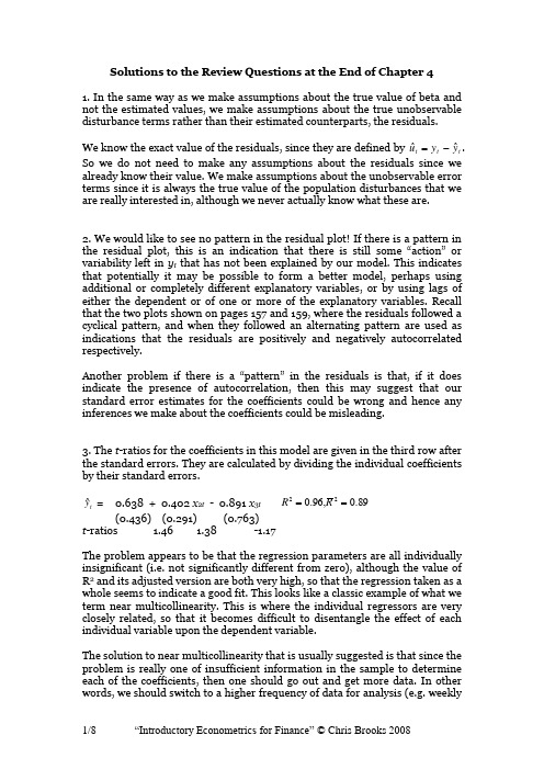
Solutions to the Review Questions at the End of Chapter 41. In the same way as we make assumptions about the true value of beta and not the estimated values, we make assumptions about the true unobservable disturbance terms rather than their estimated counterparts, the residuals.We know the exact value of the residuals, since they are defined by t t t y y uˆˆ-=. So we do not need to make any assumptions about the residuals since we already know their value. We make assumptions about the unobservable error terms since it is always the true value of the population disturbances that we are really interested in, although we never actually know what these are.2. We would like to see no pattern in the residual plot! If there is a pattern in the resi dual plot, this is an indication that there is still some “action” or variability left in y t that has not been explained by our model. This indicates that potentially it may be possible to form a better model, perhaps using additional or completely different explanatory variables, or by using lags of either the dependent or of one or more of the explanatory variables. Recall that the two plots shown on pages 157 and 159, where the residuals followed a cyclical pattern, and when they followed an alternating pattern are used as indications that the residuals are positively and negatively autocorrelated respectively.Another problem if there is a “pattern” in the residuals is that, if it does indicate the presence of autocorrelation, then this may suggest that our standard error estimates for the coefficients could be wrong and hence any inferences we make about the coefficients could be misleading.3. The t -ratios for the coefficients in this model are given in the third row after the standard errors. They are calculated by dividing the individual coefficients by their standard errors.t yˆ = 0.638 + 0.402 x 2t - 0.891 x 3t 89.0,96.022==R R (0.436) (0.291) (0.763)t -ratios 1.46 1.38 -1.17The problem appears to be that the regression parameters are all individually insignificant (i.e. not significantly different from zero), although the value of R 2 and its adjusted version are both very high, so that the regression taken as a whole seems to indicate a good fit. This looks like a classic example of what we term near multicollinearity. This is where the individual regressors are very closely related, so that it becomes difficult to disentangle the effect of each individual variable upon the dependent variable.The solution to near multicollinearity that is usually suggested is that since the problem is really one of insufficient information in the sample to determine each of the coefficients, then one should go out and get more data. In other words, we should switch to a higher frequency of data for analysis (e.g. weeklyinstead of monthly, monthly instead of quarterly etc.). An alternative is also to get more data by using a longer sample period (i.e. one going further back in time), or to combine the two independent variables in a ratio (e.g. x 2t / x 3t ).Other, more ad hoc methods for dealing with the possible existence of near multicollinearity were discussed in Chapter 4:- Ignore it: if the model is otherwise adequate, i.e. statistically and in terms of each coefficient being of a plausible magnitude and having an appropriate sign. Sometimes, the existence of multicollinearity does not reduce the t -ratios on variables that would have been significant without the multicollinearity sufficiently to make them insignificant. It is worth stating that the presence of near multicollinearity does not affect the BLUE properties of the OLS estimator – i.e. it will still be consistent, unbiased and efficient since the presence of near multicollinearity does not violate any of the CLRM assumptions 1-4. However, in the presence of near multicollinearity, it will be hard to obtain small standard errors. This will not matter if the aim of the model-building exercise is to produce forecasts from the estimated model, since the forecasts will be unaffected by the presence of near multicollinearity so long as this relationship between the explanatory variables continues to hold over the forecasted sample.- Drop one of the collinear variables - so that the problem disappears. However, this may be unacceptable to the researcher if there were strong a priori theoretical reasons for including both variables in the model. Also, if the removed variable was relevant in the data generating process for y , an omitted variable bias would result.- Transform the highly correlated variables into a ratio and include only the ratio and not the individual variables in the regression. Again, this may be unacceptable if financial theory suggests that changes in the dependent variable should occur following changes in the individual explanatory variables, and not a ratio of them.4. (a) The assumption of homoscedasticity is that the variance of the errors isconstant and finite over time. Technically, we write 2)(u t u Var σ=.(b ) The coefficient estimates would still be the “correct” ones (assuming that the other assumptions required to demonstrate OLS optimality are satisfied), but the problem would be that the standard errors could be wrong. Hence if we were trying to test hypotheses about the true parameter values, we could end up drawing the wrong conclusions. In fact, for all of the variables except the constant, the standard errors would typically be too small, so that we would end up rejecting the null hypothesis too many times.(c) There are a number of ways to proceed in practice, including- Using heteroscedasticity robust standard errors which correct for the problem by enlarging the standard errors relative to what they would havebeen for the situation where the error variance is positively related to one of the explanatory variables.- Transforming the data into logs, which has the effect of reducing the effect of large errors relative to small ones.5. (a) This is where there is a relationship between the i th and j th residuals. Recall that one of the assumptions of the CLRM was that such a relationship did not exist. We want our residuals to be random, and if there is evidence of autocorrelation in the residuals, then it implies that we could predict the sign of the next residual and get the right answer more than half the time on average!(b) The Durbin Watson test is a test for first order autocorrelation. The test is calculated as follows. You would run whatever regression you were interested in, and obtain the residuals. Then calculate the statistic()∑∑==--=T t t T t t t uuu DW 22221ˆˆˆYou would then need to look up the two critical values from the Durbin Watson tables, and these would depend on how many variables and how many observations and how many regressors (excluding the constant this time) you had in the model.The rejection / non-rejection rule would be given by selecting the appropriate region from the following diagram:(c) We have 60 observations, and the number of regressors excluding the constant term is 3. The appropriate lower and upper limits are 1.48 and 1.69 respectively, so the Durbin Watson is lower than the lower limit. It is thus clear that we reject the null hypothesis of no autocorrelation. So it looks like the residuals are positively autocorrelated.(d) t t t t t u x x x y +∆+∆+∆+=∆4433221ββββThe problem with a model entirely in first differences, is that once we calculate the long run solution, all the first difference terms drop out (as in the long run we assume that the values of all variables have converged on their own long run values so that y t = y t -1 etc.) Thus when we try to calculate the long run solution to this model, we cannot do it because there isn’t a long run solution to this model!(e) t t t t t t t t v X X x x x x y ++++∆+∆+∆+=∆---1471361254433221βββββββThe answer is yes, there is no reason why we cannot use Durbin Watson in this case. You may have said no here because there are lagged values of the regressors (the x variables) variables in the regression. In fact this would be wrong since there are no lags of the DEPENDENT (y ) variable and hence DW can still be used.6. t rt t t t t t t u x x x y x x y +++++∆+∆+=∆----471361251433221βββββββThe major steps involved in calculating the long run solution are to- set the disturbance term equal to its expected value of zero- drop the time subscripts- remove all difference terms altogether since these will all be zero by the definition of the long run in this context.Following these steps, we obtain373625410x x x y βββββ++++=We now want to rearrange this to have all the terms in x 2 together and so that y is the subject of the formula:344624541376251437362514)()(x x y x x y x x x y βββββββββββββββββ+---=+---=----=The last equation above is the long run solution.7. Ramsey’s RESET test is a test of whether the functional form of the regression is appropriate. In other words, we test whether the relationship between the dependent variable and the independent variables really should be linear or whether a non-linear form would be more appropriate. The test works by adding powers of the fitted values from the regression into a secondregression. If the appropriate model was a linear one, then the powers of the fitted values would not be significant in this second regression.If we fail Ramsey’s RESET test, then the easiest “solution” is probably to transform all of the variables into logarithms. This has the effect of turning a multiplicative model into an additive one.If this still fails, then we really have to admit that the relationship between the dependent variable and the independent variables was probably not linear after all so that we have to either estimate a non-linear model for the data (which is beyond the scope of this course) or we have to go back to the drawing board and run a different regression containing different variables.8. (a) It is important to note that we did not need to assume normality in order to derive the sample estimates of αand βor in calculating their standard errors. We needed the normality assumption at the later stage when we come to test hypotheses about the regression coefficients, either singly or jointly, so that the test statistics we calculate would indeed have the distribution (t or F) that we said they would.(b) One solution would be to use a technique for estimation and inference which did not require normality. But these techniques are often highly complex and also their properties are not so well understood, so we do not know with such certainty how well the methods will perform in different circumstances.One pragmatic approach to failing the normality test is to plot the estimated residuals of the model, and look for one or more very extreme outliers. These would be residuals that are much “bigger” (either very big and positive, or very big and negative) than the rest. It is, fortunately for us, often the case that one or two very extreme outliers will cause a violation of the normality assumption. The reason that one or two extreme outliers can cause a violation of the normality assumption is that they would lead the (absolute value of the) skewness and / or kurtosis estimates to be very large.Once we spot a few extreme residuals, we should look at the dates when these outliers occurred. If we have a good theoretical reason for doing so, we can add in separate dummy variables for big outliers caused by, for example, wars, changes of government, stock market crashes, changes in market microstructure (e.g. the “big bang” of 1986). The effect of the dummy variable is exactly the same as if we had removed the observation from the sample altogether and estimated the regression on the remainder. If we only remove observations in this way, then we make sure that we do not lose any useful pieces of information represented by sample points.9. (a) Parameter structural stability refers to whether the coefficient estimates for a regression equation are stable over time. If the regression is not structurally stable, it implies that the coefficient estimates would be different for some sub-samples of the data compared to others. This is clearly not what we want to find since when we estimate a regression, we are implicitly assuming that the regression parameters are constant over the entire sample period under consideration.(b) 1981M1-1995M12r t = 0.0215 + 1.491 r mt RSS =0.189 T =1801981M1-1987M10r t = 0.0163 + 1.308 r mt RSS =0.079 T =821987M11-1995M12r t = 0.0360 + 1.613 r mt RSS =0.082 T =98(c) If we define the coefficient estimates for the first and second halves of the sample as α1 and β1, and α2 and β2 respectively, then the null and alternative hypotheses areH 0 : α1 = α2 and β1 = β2and H 1 : α1 ≠ α2 or β1 ≠ β2(d) The test statistic is calculated asTest stat. =304.1524180*082.0079.0)082.0079.0(189.0)2(*)(2121=-++-=-++-k k T RSS RSS RSS RSS RSSThis follows an F distribution with (k ,T -2k ) degrees of freedom. F (2,176) = 3.05 at the 5% level. Clearly we reject the null hypothesis that the coefficients are equal in the two sub-periods.10. The data we have are1981M1-1995M12r t = 0.0215 + 1.491 R mt RSS =0.189 T =1801981M1-1994M12r t = 0.0212 + 1.478 R mt RSS =0.148 T =1681982M1-1995M12r t = 0.0217 + 1.523 R mt RSS =0.182 T =168First, the forward predictive failure test - i.e. we are trying to see if the model for 1981M1-1994M12 can predict 1995M1-1995M12.The test statistic is given by832.3122168*148.0148.0189.0*2111=--=--T k T RSS RSS RSSWhere T 1 is the number of observations in the first period (i.e. the period that we actually estimate the model over), and T 2 is the number of observations we are trying to “predict”. The test statistic follows an F -distribution with (T 2, T 1-k ) degrees of freedom. F (12, 166) = 1.81 at the 5% level. So we reject the null hypothesis that the model can predict the observations for 1995. We would conclude that our model is no use for predicting this period, and from a practical point of view, we would have to consider whether this failure is a result of a-typical behaviour of the series out-of-sample (i.e. during 1995), or whether it results from a genuine deficiency in the model.The backward predictive failure test is a little more difficult to understand, although no more difficult to implement. The test statistic is given by532.0122168*182.0182.0189.0*2111=--=--T k T RSS RSS RSSNow we need to be a little careful in our interpretation of what exactly are the “first” and “second” sample periods. It would be possible to define T 1 as always being the first sample period. But I think it easier to say that T 1 is always the sample over which we estimate the model (even though it now comes after the hold-out-sample). Thus T 2 is still the sample that we are trying to predict, even though it comes first. You can use either notation, but you need to be clear and consistent. If you wanted to choose the other way to the one I suggest, then you would need to change the subscript 1 everywhere in the formula above so that it was 2, and change every 2 so that it was a 1.Either way, we conclude that there is little evidence against the null hypothesis. Thus our model is able to adequately back-cast the first 12 observations of the sample.11. By definition, variables having associated parameters that are not significantly different from zero are not, from a statistical perspective, helping to explain variations in the dependent variable about its mean value. One could therefore argue that empirically, they serve no purpose in the fitted regression model. But leaving such variables in the model will use up valuable degrees of freedom, implying that the standard errors on all of the other parameters in the regression model, will be unnecessarily higher as a result. If the number of degrees of freedom is relatively small, then saving a couple by deleting two variables with insignificant parameters could be useful. On the other hand, if the number of degrees of freedom is already very large, the impact of these additional irrelevant variables on the others is likely to be inconsequential.12. An outlier dummy variable will take the value one for one observation in the sample and zero for all others. The Chow test involves splitting the sample into two parts. If we then try to run the regression on both the sub-parts butthe model contains such an outlier dummy, then the observations on that dummy will be zero everywhere for one of the regressions. For that sub-sample, the outlier dummy would show perfect multicollinearity with the intercept and therefore the model could not be estimated.。

第⼀章委托代理（纽约⼤学艾伦和盖尔⾦融经济学讲义）Chapter1The principal-agent problemThe principal-agent problem describes a class of interactions between two parties to a contract,an agent and a principal.The legal origin of these terms suggests that the principal engages the agent to act on his(the principal’s) behalf.In economic applications,the agent is not necessarily an employe of the principal.In fact,which of two individuals is regarded as the agent and which as the principal depends on the nature of the incentive problem. Typically,the agent is the one who is in a position to gain some advantage by reneging on the agreement.The principal then has to provide the agent with incentives to abide by the terms of the contract.We divide principal-agent problems into two classes:problems of hidden action and problems of hidden information.In hidden-action problems,the agent takes an action on behalf of the principal.The principal cannot observe the action directly,however,so he has to provide incentives for the agent to choose the action that is best for the principal.In hidden-information prob-lems,the agent has some private information that is needed for some decision to be made byprincipal.Again,since the principal cannot observe the agent’s information,he has to provide incentives for the agent to reveal the infor-mation truthfully.We begin by looking at the hidden-action problem,also known as a moral hazard problem.1.1The modelFor concreteness,imagine that the principal and the agent undertake a risky venture together and agree to share the revenue.The agent takes some12CHAPTER1.THE PRINCIPAL-AGENT PROBLEM action that a?ects the outcome of the project.The revenue from the venture is assumed to be a random function of the agent’s action.Let A denote the set of actions available to the agent with generic element a.Typically,A is either a?nite set or an interval of real numbers.Let S denote a set of states with generic element s.For simplicity,we assume that the set S is?nite.The probability of the state s conditional on the action a is denoted by p(a,s).The revenue in state s is denoted by R(s)≥0.The agent’s utility depends on both the action chosen and the consump-tion he derives from his share of the revenue.The principal’s utility depends only on his consumption.We maintain the following assumptions about preferences:The agent’s utility function u:A×R+→R is additively separable:u(a,c)=U(c)?ψ(a).Further,the function U:R+→R is C2and satis?es U0(c)>0and U00(c)≤0.The principal’s utility function V:R→R is C2and satis?es V0(c)>0 and V00(c)≤0.Notice that the agent’s consumption is assumed to be non-negative.This is interpreted as a liquidity constraint or limited liability.The principal’s consumption is not bounded below;in some contexts this is equivalent to assuming that the principal has large but?nite wealth and non-negative consumption.1.2Pareto e?ciencyThe principal and the agent jointly choose a contract that speci?es an action and a division of the revenue.A contract is an ordered pair(a,w(·))∈A×W, where W={w:S→R+}is the set of incentive schemes and w(s)≥0is the payment to the agent in state s.Suppose that all variables are observable and veri?able.The principal and the agent will presumably choose a contract that is Pareto-e?cient. This leads us to consider the following decision problem(DP1):max(a,w(·))X s∈S p(a,s)V(R(s)?w(s))1.3.INCENTIVE EFFICIENCY3 subject to X s∈S p(a,s)U(w(s))?ψ(a)≥¯u,for some constant¯u.Proposition1Under the maintained assumptions,a contract(a,w(·))is Pareto-e?cient if and only if it is a solution to the decision problem DP1for some¯u.Suppose that(a,w(·))is Pareto-e?cient.Put¯u equal to the agent’s pay-o?.By de?nition,the contract must maximize the principal’s payo?subject to the constraint that the agent receive at least¯u.Conversely,suppose that the contract(a,w(·))is a solution to DP1for some value of¯u.If the contract is not Pareto-e?cient,then there must be another contract that yields the same payo?to the principal and more to the agent.But then it must be possible to transfer wealth to the principal in some state,contradicting the optimality of(a,w(·)).Suppose that the sharing rule satis?es w(s)>0for all s.Then optimal risk sharing requires:V0(R(s)?w(s))=λ,?s.These are sometimes referred to as the Borch conditions.If the action a belongs to the interior of A and if the functionsp(a,s)andψ(a)are di?er-entiable at a,thenX s∈S p a(a,s)[V(R(s)?w(s))?λU(w(s)]+λψ0(a)=0.1.3Incentive e?ciencyNow suppose that the agent’s action is neither observable nor veri?able.In that case,the action speci?ed by the contract must be consistent with the agent’s incentives.A contract(a,w(·))is incentive-compatible if it satis?es the constraintX s∈S p(a,s)U(w(s))?ψ(a)≥X s∈S p(b,s)U(w(s))?ψ(b),?b.4CHAPTER1.THE PRINCIPAL-AGENT PROBLEM A contract is incentive-e?cient if it is incentive-compatible and there does not exist another incentive-compatible contract that makes one party bet-ter o?without making the other party worse o?.We can characterize the incentive-e?cient contracts using the following decision problem(DP2):max(a,w(·))X s∈S p(a,s)V(R(s)?w(s))subject toX s∈S p(a,s)U(w(s))?ψ(a)≥X s∈S p(b,s)U(w(s))?ψ(b),?b, and X s∈S p(a,s)U(w(s))?ψ(a)≥¯u.Proposition2Under the maintained assumptions,a contract(a,w(·))is incentive-e?cient only if it is a solution of DP2for some constant¯u.A contract that solves DP2is incentive-e?cient if the participation constraint is binding for every solution.The proof of the“only if”part is similar to the Pareto e?ciency argument. If(a,w(·))is a solution to DP2and is not incentive-e? cient,there exists an incentive-e?cient contract that gives the principal the same payo?and the agent a higher payo?.But this contract must be a solution to DP2that strictly satis?es the participation constraint.The assumption of a uniformly binding participation constraint is restric-tive:see Section1.7.1for a counter-example.This DP can be solved in two stages.First,for any action a,compute the payo?V?(a)from choosing a and providing optimal incentives to the agent to choose a.Call this DP3V?(a)=maxw(·)X s∈S p(a,s)V(R(s)?w(s))subject toX s∈S p(a,s)U(w(s))?ψ(a)≥X s∈S p(b,s)U(w(s))?ψ(b),?b, X s∈S p(a,s)U(w(s))?ψ(a)≥¯u.1.4.THE IMPACT OF INCENTIVE CONSTRAINTS5Note that U(·)and V(·)are concave functions.A suitable transformation of this problem(see Section1.10)is a convex programming problem for which the Kuhn-Tucker conditions are necessary and su?cient.Once the function V?is determined,the optimal action is chosen to max-imize the principal’s payo?:a?∈arg max V?(a).The advantage of the two-stage procedure is that it allows us to focus on the problem of implementing a particular action.DP3is(equivalent to)a convex programming problem and hence easier to“solve”and it turns out that many interesting properties can be derived from a study of DP3without worrying about the optimal choice of action.1.3.1Risk neutralityAn interesting special case arises if the principal is risk neutral.In that case,maximization of the principal’s expected utility,taking a as given,is equivalent to minimizing the cost of the payments to the agent.Thus,DP3 can be re-written asminw(·)X s∈S p(a,s)w(s))subject toX s∈S p(a,s)U(w(s))?ψ(a)≥X s∈S p(b,s)U(w(s))?ψ(b),?b, X s∈S p(a,s)U(w(s))?ψ(a)≥¯u.1.4The impact of incentive constraintsWhat is the impact of hidden information?When does the imposition in-centive constraints a?ect the choice of contract?If one of the parties to the contract is risk neutral,it is particularly easy to check whether the?rst best can be achieved,that is,whether an incentive-e?cient contract is also Pareto-e?cient.Suppose,for example,that the principal is risk neutral and the agent is(strictly)risk averse,i.e.,U00(c)<0. The Borch conditions for an interior solution imply that w(s)is a constant6CHAPTER1.THE PRINCIPAL-AGENT PROBLEM for all s.In that case,the agent’s income is independent of his action,so in the hidden action case he would choose the cost-minimizing action.Thus, the?rst best can be achieved with hidden actions only if the optimal action is cost-minimizing.Suppose that the agent is risk neutral and the principal is(strictly)risk averse,i.e.,V00(c)<0.Then the Borch conditions for the? rst best imply that the principal’s income R(s)?w(s)is constant,as long as the solution is interior.This corresponds to the solution of“selling the?rm to the agent”, but it works only as long as the agent’s non-negative consumption constraint is not binding.In general,there is some constant¯y such thatR(s)?w(s)=min{¯y,R(s)}andw(s)=max{R(s)?¯y,0}.More generally,if we assume the?rst best is an interior solution and maintain the di?erentiability assumptions discussed above,the?rst-order condition for the?rst best isX s∈S p a(a,s)[V(R(s)?w(s))?λU(w(s)]+λψ0(a)=0.and the?rst-order(necessary)condition for the incentive-compatibility con-straint is X s∈S p a(a,s)[U(w(s)]?ψ0(a)=0.So the incentive-e?cient and?rst-best contracts coincide only ifX s∈S p a(a,s)V(R(s)?w(s))=0.Note that there may be no interior solution of the problem DP3even under the usual Inada conditions.See Section1.7.2for a counter-example.1.5The optimal incentive schemeIn order to characterize the optimal incentive scheme more completely,we impose the following assumptions:1.5.THE OPTIMAL INCENTIVE SCHEME7?The principal is risk neutral,which means that if two actions are equally costly to implement,he will always prefer the one that yields higher expected revenue.There is anite number of states s=1,...,S and the revenue function R(s)is increasing in s.Monitone likelihood ratio property:There is anite number of actions a=1,...,A and for any actions aNow consider the modi?ed DP4of implementing a?xed value of a:w(·)X s∈S p(a,s)V(R(s)?w(s))subject toX s∈S p(a,s)U(w(s))?ψ(a)≥X s∈S p(b,s)U(w(s))?ψ(b),?bThe di?erence between DP4and the original DP3is that only the downward incentive constraints are included.Obviously,V??(a)≥V?(a).Suppose that V??(a)>V?(a).This means that the agent wants to choose a higher action than a in the modi?ed problem. But this is good for the principal,who will never choose a if he can get a better action for the same price.Thus,maxa V?(a)=maxaV??(a).Thus,we can use the solution to the modi?ed problem DP4to characterize the optimal incentive scheme.Theorem3Suppose that a∈arg max V?(a).The incentive scheme w(·)is a solution of DP4if and only if it is a solution of DP3.8CHAPTER1.THE PRINCIPAL-AGENT PROBLEM1.6MonotonicityMany incentive schemes observed in practice reward the agent with higherrewards for higher outcomes,i.e.,w(s)is increasing(or non-decreasing)in s.It is interesting to see when this is a property of the theoretical optimal in-centive scheme.Assuming an interior solution,the Kuhn-Tucker(necessary)conditions are:p(a,s)V0(R(s)?w(s))?λp(a,s)U0(w(s))?X borV0(R(s)?w(s))=?λ+X bU0(w(s))By the MLRP,the right hand side is non-increasing in s,so the left handside is non-increasing,which means that w(s)is non-decreasing.1.7ExamplesThere are two outcomes s=1,2,where R(1)a=1,2represented by the respective probabilities of success0p(2,2)<1.The costs of e?ort areψ(1)=0andψ(2)>0.The agent’s utilityfunction U(·)is assumed to satisfy U(0)=0and the reservation utility is¯u=0.The inferior project can be implemented by setting w(s)=0for s=1,2.Suppose the principal wants to implement a=2.The constraints can be(IC)(1?p(2,2))U(w(1))+p(2,2)U(w(2))?ψ(2)≥(1?p(1,2))U(w(1))+p(1,2)U(w(2)) which simpli?es to(p(2,2)?p(1,2))(U(2)?U(1))≥ψ(2)and(IR)(1?p(2,2))U(w(1))+p(2,2)U(w(2))?ψ(2)≥0.In order to satisfy the(IR)constraint,consumption must be positive in atleast one state.This implies that the expected utility from choosing lowe?ort is strictly positive:(1?p(1,2))U(w(1))+p(1,2)U(w(2))>0,1.7.EXAMPLES9 so if the(IC)constraint is satis?ed,the(IR)constraint must be strictly satis?ed:(1?p(2,2))U(w(1))+p(2,2)U(w(2))?ψ(2)>0.Thus,if(w(1),w(2))is the solution to the optimal contract problem,the (IR)constraint does not bind.The principal’s problem can then be written as:min w(1?p(2,2))w(1)+p(2,2)w(2)s.t.(w(1),w(2)≥0(p(2,2)?p(1,2))(U(w(2))?U(w(1)))≥ψ(2).Then it is clear that a necessary condition for an optimum is that w(1)=0. So the optimal contract for implementing a=2is(0,w?(2)),where w?(2) solves the(IC):(p(2,2)?p(1,2))U(w?(2))=ψ(2).The payment w?(2)needed to give the necessary incentives to the manager will be higher:the higher the cost of eortψ(2);the smaller the manager’s risk tolerance(as measured by U(w(2))U(0));the smaller the marginal productivity of eort(as measured by p(2,2)p(1,2)).To decide whether it is optimal to implement high or low e?ort,the prin-cipal compares the pro?t from optimally implementing each level of e?ort. The maximum pro?t from low e?ort is(1?p(1,2))R(2)+p(1,2)R(1).The maximum pro?t from high e?ort is(1?p(2,2))R(1)+p(2,2)R(2)?p(2,2)w?(2).So high e?ort is optimal if and only if(p(2,2)?p(1,2))(R(2)?R(1))≥w?(2),that is,the increase in expected revenue is greater than the cost of providing managerial incentives.10CHAPTER1.THE PRINCIPAL-AGENT PROBLEM 1.7.1Optimality and incentive-e?ciencySuppose there are two states s=1,2,two actions a=1,2and the reservation utility is¯u=0.The principal and the agent are both risk neutral.The other parameters of the problem are given byR(1)=0ψ(1)=0<ψ(2)The action a=1is optimally implemented by puttingw1(s)=0,?s.The action a=2is optimally implemented by puttingw2(s)=?0if s=1ψ(2)/(p(2,2)?p(1,2))if s=2.The payo?to the principal from each action isV?(a)=?p(1,2)R(2)if a=1p(2,2)(R(2)?ψ(2)/(p(2,2)?p(1,2)))if a=2. Suppose the parameter values are chosen so that V?(1)=V?(2).Then thecontract(a,w(·))=(1,w1(·))solves DP1for the reservation utility¯u=0 but is not incentive e?cient,because the agent is better o? with the contract (a,w(·))=(2,w2(·)).1.7.2Boundary solutionsIn the preceding example,we note that the agent’s payo?is zero in state s=0 whichever action is implemented.It might be thought that this boundary solution is dependent on risk neutrality but in fact boundary solutions for optimal incentive scheme are possible even if U0(0)=∞,for example,for the utility function U(c)=cαwhere0<α<1.In this case,U(0)=0so, taking the other parameters from the previous example,the optimal incentive scheme for a=1is stillw1(s)=0,?s.1.7.EXAMPLES11 For a=2the optimal incentive scheme isw2(s)=?0if s=1U?1(ψ(2)/(p(2,2)?p(1,2)))if s=2.This example provides a good illustration of the dangers of simply assuming an interior solution.1.7.3Local incentive constraintsIn many problems,convexity implies that one only has to consider local deviations in order to characterize an optimum.The analogous principle in principal-agent problems is to check only local incentive constraints.For example,if a=1,...,A and it is desired to implement an action a then one would only check the neighboring constraints a?1and a+1(or in the case where only downward constraints are considered,one would look at the constraint between a and a?1only).There is in general no reason to think that this method will produce the right answer:there may well be non-local constraints that are binding at the optimum.For example,suppose that there are two states s=1,2and three actions a=1,2,3.The principal and the agent are both assumed to be risk neutral and the reservation utility is ¯u=0.The other parameters are as follows:R(1)=0ψ(1)=0<ψ(2)=ψ(3)The optimal incentive scheme to implement a=3isw3(s)=?0if s=1(ψ(3)/(p(2,2)?p(1,2)))if s=2.Because a=2has the same cost but lower probability of success than a=3, the agent will never be tempted to choose a=2as long as the payment in state s=2is positive;but he may well be tempted to choose a=1if the payment in state s=2is too low.Thus,the incentive constraint between a=1and a=3will be binding but the incentive constraint between a=3 and a=2will not.12CHAPTER1.THE PRINCIPAL-AGENT PROBLEM To ensure that the local constraint was su?cient,we would need to impose the following inequality on the parameters:p(3,2)?p(2,2)ψ(3)?ψ(2)≤p(2,2)?p(1,2)ψ(2)?ψ(1).This is,in e?ect,an assumption of diminishing returns to scale:the marginalproduct of e?ort as measured by the ratio of the change in the probability ofsuccess to the change in cost is declining.In more general problems,strongerconditions are needed to ensure that only local incentive constraints bind.See,for example,the discussion of the?rst-order approach in Stole(2001).1.7.4Participation constraints1.8The value of informationThe principal may observe some information that is relevant to the agent’saction in addition to the revenue from the project.We can incorporate thispossibility in the current setup by assuming that the state is an ordered pairs=(s1,s2)∈S1×S2and that the revenue is a function R(s1)of the?rst component.Then s2is a pure signal of the action a.The? rst-order conditionfor an interior solution to DP4isV0(R(s1,s2)?w(s1,s2))12=?λ+X bThe state s2gives information about the action of the principal if the like-lihood ratio p(b,s1,s2)/p(a,s1,s2)varies with s2for some?xed s1.In other words,all relevant information should be re?ected in the agent’s payment.1.9Mechanism designThe principal-agent problem is a special case of the general problem of mech-anism design,that is,designing a game form that will implement a desired outcome as an equilibrium of the game.Suppose there is a?nite number of agents i=1,...,I,each of whom has a typeθi∈Θi and chooses an action a i∈A i.There may also be a set of actions a0∈A0chosen by the mechanism designer.LetΘ=Q I i=1Θi and A=Q I i=0A i and denote elements ofΘand1.9.MECHANISM DESIGN13A byθand a respectively.An agent’s utility is given by u i(a,θ),that is,u i:A×Θ→R.An agent’s type is private information,but the distribution of types p(θ)is common knowledge,as are the setsΘi and A i and the utility functions u i.The mechanism designer faces two problems:how to get the agents toreveal their information truthfully and how to get them to choose the“right”actions.The general form of a mechanism contains two stages:in the?rstagents are asked to send messages to the planner and in the second theplanner sends instructions to the agents.Let M i denote the space of messagesavailable to agent i and let M=Q i M i.Let M0denote the planner’s message space and f:M→M0denote the decision rule chosen by the planner.Theneach agent has to choose a strategy(σi,αi),whereσi:Θi→Θi andαi: M0→A i.Given f we have a well-de?ned game with players is i=1,...,I, strategy sets{Σi}I i=1and payo?functions{U i}I i=1,where U i:Σ→R is de?ned byU i(σ,α,θ)=u i(α?f?σ(θ),θ).A Bayes-Nash equilibrium for this game is a strategy pro?le(,σ?,α?)such that,for every agent i,E[U i(σ,α,θ)|θi]≥E[U i((σi,αi),(σ?i,αi),θ)|θi],?θi,?(σi,αi).A mechanism(f,M)is called a direct mechanism if M i=Θi for i=1,...,I and M0=A.In other words,agents’messages are their types andthe planner’s message is the vector of desired actions.For any agent i,thetruthful communication strategy in a direct mechanism is a communicationstrategyσi such thatσi(θi)=θi,?θi.Similarly,in a direct mechanism,an action strategyαi is truthful ifαi(a)=a i,?a∈A.The Revelation Principle allows us to substitute direct mechanisms for gen-eral mechanisms and restrict attention to truthful strategies.Theorem4(RevelationP rinciple)Let(σ,α)be a Bayes-Nash equilibriumof the mechanism(f,M).Then there exists a Bayes-Nash equilibrium(?σ,?α)of the direct mechanism(?f,Θ)such that(?σi,?αi)are truthful for every i andthe outcomes of the two equilibria are the same:α?f?σ=?α??f??σ.14CHAPTER1.THE PRINCIPAL-AGENT PROBLEM Proof.Put?f=α?f?σ.Although the proof is trivial,this result o?ers a great simpli?cation of the problem of characterizing implementable SCFs.A SCF is a function f:Θ→A that speci?es an outcome for every state of natureθ.We can think of the SCF f as a collection of decision rules(f0,f1,...,f I),one for each agent i.The SCF f is incentive-compatible if,for every i,truth-telling is optimal and the decision rule f i is optimal,assuming that every other agent j tells the truth and follows the decision rule f j,that is,E[u i(f(θ),θ)|θi]≥E h u i3a i,f?i(?θi,θ?i),θ′|θi i.Theorem5The direct mechanism(f,Θ)has a truthful equilibrium if and only if f is an incentive-compatible SCF.Remark1The theorem suggests that we can“implement”f using a direct mechanism,but the direct mechanism may have other equilibrium.Full im-plementation requires that every equilibrium of the mechanism used have the same outcome.For this it may be necessary to use a general mechanism. Most of the implementation literature is taken up with this problem of try-ing to eliminate unwanted equilibria,either by using fancier mechanisms or stronger solution concepts.Remark2The principal-agent problem is a special kind of mechanism de-sign problem.In the problem described earlier,there are two“agents”(the principal and the agent both being economic agents in the eyes of the mech-anism designer).The agent chooses an action a∈A,the principal has no action to choose,and the mechanism designer chooses the incentive scheme w(·)∈W.Since there is no private information about types,the SCF is an incentive-e?cient allocation f=(a,w(·))and the direct mechanism has a truthful equilibrium in which the agent chooses the correct value of a.Even in this simple context we can see the problem of multiple equilibria at work. Typically,the incentive scheme is chosen so that the agent is indi?erent be-tween a and some other action b.It would be an equilibrium for the agent to choose b even though this would not be as good for the principal.We can use this example to illustrate how a more complex mechanism and a stronger equilibrium concept helps resolve this di?culty.Suppose that the principal is told to choose the incentive scheme and that the agent chooses his action after observing the incentive scheme.The appropriate solution concept here1.10.NON-CONVEXITY AND LOTTERIES15 is subgame perfect equilibrium:the agent should choose the best response (action)to any incentive scheme and not simply the one that is chosen in equlibrium.Clearly,the truthful equilibriumof(a,w(·))remains a SPE of this game but(b,w(·))does not.If the principal anticipates that the agent will choose b under the incentive scheme w(·)and if the principal prefers a to b,then he will choose an alternative?w(·)which is very close to w(·)but makes the agent strictly prefer a to b.Thus,(b,w(·))is not a SPE.Remark3The sequential game described above,in which the principal of-fers an incentive scheme and the agent responds optimally to any scheme o?ered,is closer to the original formulation of the principal-agent problem than the decision problems analyzed above.We have taken an approach much closer to the Revelation Principal,in which we focus exclusively on the truth-ful equilibria.Within the context of mechanism design,we can see that both approaches are closely related.1.10Non-convexity and lotteriesThe principal-agent problem as stated earlier is not a convex programming problem because the feasible set de?ned by the incentive constraints is not convex:X s∈S p(a,s)U(w(s))?ψ(a)≥X s∈S p(b,s)U(w(s))?ψ(b),?bThe concave function U(·)appears on both sides of the inequality.However, a simple transformation suggested by Grossman and Hart converts this into a convex programming problem.Let C(u)=U?1(u)for any number u.C(·)is convex because U(·)is concave and we can write the implementation problemequivalently asminu(·)X s∈S p(a,s)V(R(s)?C(u(s)))subject toX s∈S p(a,s)u(s)?ψ(a)≥X s∈S p(b,s)u(s)?ψ(b),?b,X s∈S p(a,s)u(s))?ψ(a)≥¯u.16CHAPTER1.THE PRINCIPAL-AGENT PROBLEM Because the incentive scheme u(s)is written in terms of utility rather than consumption,the incentive constraints are linear in the choice variables and hence the feasible set is convex.This trick works because of the additive separability of the utility func-tion.In general,this will not work and we are stuck with a highly non-convex problem.One general solution to non-convexities is to introduce lotteries. Let the incentive scheme specify a probability distribution W(c,s)over non-negative consumption levels c conditional on the state s and let the utility function take the general form u(c,a).The incentive constraint is then writ-ten as X s∈S[p(a,s)?p(b,s)]u(c,a)W(dc,s)≥0,?b.Expected utility is linear in probabilites,so once again the incentive con-straints de?ne a convex feasible set of distributions W(·).Lotteries are not simply a solution to a technical problem(non-convexity).They can also increase welfare.Note that even if the implementation problem does not include non-convexities because of the additive separability of preferences,the global principal agent problem may do so because the cost functionψis non-convex. Although each action a can be implemented e?ciently with a non-stochastic incentive scheme,there may be a gain from randomizing over the action a.。