伍德里奇《计量经济学导论》(第4版)笔记和课后习题详解-第1~4章【圣才出品】

《计量经济学导论》考研伍德里奇考研复习笔记二第1章计量经济学的性质与经济数据1.1 复习笔记一、什么是计量经济学计量经济学是以一定的经济理论为基础，运用数学与统计学的方法，通过建立计量经济模型，定量分析经济变量之间的关系。

在进行计量分析时，首先需要利用经济数据估计出模型中的未知参数，然后对模型进行检验，在模型通过检验后还可以利用计量模型来进行预测。

在进行计量分析时获得的数据有两种形式，实验数据与非实验数据：（1）非实验数据是指并非从对个人、企业或经济系统中的某些部分的控制实验而得来的数据。

非实验数据有时被称为观测数据或回顾数据，以强调研究者只是被动的数据搜集者这一事实。

（2）实验数据通常是通过实验所获得的数据，但社会实验要么行不通要么实验代价高昂，所以在社会科学中要得到这些实验数据则困难得多。

二、经验经济分析的步骤经验分析就是利用数据来检验某个理论或估计某种关系。

1．对所关心问题的详细阐述问题可能涉及到对一个经济理论某特定方面的检验，或者对政府政策效果的检验。

2构造经济模型经济模型是描述各种经济关系的数理方程。

3经济模型变成计量模型先了解一下计量模型和经济模型有何关系。

与经济分析不同，在进行计量经济分析之前，必须明确函数的形式，并且计量经济模型通常都带有不确定的误差项。

通过设定一个特定的计量经济模型，我们就知道经济变量之间具体的数学关系，这样就解决了经济模型中内在的不确定性。

在多数情况下，计量经济分析是从对一个计量经济模型的设定开始的，而没有考虑模型构造的细节。

一旦设定了一个计量模型，所关心的各种假设便可用未知参数来表述。

4搜集相关变量的数据5用计量方法来估计计量模型中的参数，并规范地检验所关心的假设在某些情况下，计量模型还用于对理论的检验或对政策影响的研究。

三、经济数据的结构1横截面数据（1）横截面数据集，是指在给定时点对个人、家庭、企业、城市、州、国家或一系列其他单位采集的样本所构成的数据集。

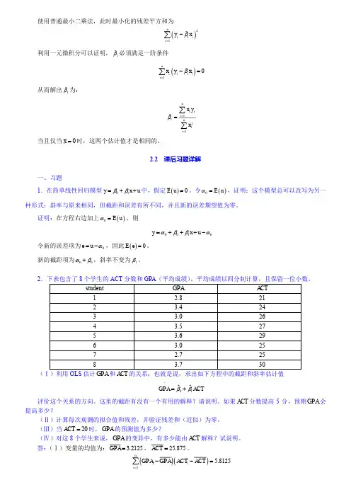
使用普通最小二乘法，此时最小化的残差平方和为()211niii y x β=-∑利用一元微积分可以证明，1β必须满足一阶条件()110niiii x y x β=-=∑从而解出1β为：1121ni ii nii x yxβ===∑∑当且仅当0x =时，这两个估计值才是相同的。

2.2 课后习题详解一、习题1．在简单线性回归模型01y x u ββ=++中，假定()0E u ≠。

令()0E u α=，证明：这个模型总可以改写为另一种形式：斜率与原来相同，但截距和误差有所不同，并且新的误差期望值为零。

证明：在方程右边加上()0E u α=，则0010y x u αββα=+++-令新的误差项为0e u α=-，因此()0E e =。

新的截距项为00αβ+，斜率不变为1β。

2（Ⅰ）利用OLS 估计GPA 和ACT 的关系；也就是说，求出如下方程中的截距和斜率估计值01ˆˆGPA ACT ββ=+＾评价这个关系的方向。

这里的截距有没有一个有用的解释？请说明。

如果ACT 分数提高5分，预期GPA 会提高多少？（Ⅱ）计算每次观测的拟合值和残差，并验证残差和（近似）为零。

（Ⅲ）当20ACT =时，GPA 的预测值为多少？（Ⅳ）对这8个学生来说，GPA 的变异中，有多少能由ACT 解释？试说明。

答：（Ⅰ）变量的均值为： 3.2125GPA =，25.875ACT =。

()()15.8125niii GPA GPA ACT ACT =--=∑根据公式2.19可得：1ˆ 5.8125/56.8750.1022β==。

根据公式2.17可知：0ˆ 3.21250.102225.8750.5681β=-⨯=。

因此0.56810.1022GPA ACT =+＾。

此处截距没有一个很好的解释，因为对样本而言，ACT 并不接近0。

如果ACT 分数提高5分，预期GPA 会提高0.1022×5=0.511。

（Ⅱ）每次观测的拟合值和残差表如表2-3所示：根据表可知，残差和为-0.002，忽略固有的舍入误差，残差和近似为零。

伍德里奇-计量经济学(第4版)答案计量经济学答案第二章2.4 (1)在实验的准备过程中，我们要随机安排小时数，这样小时数（hours ）可以独立于其它影响SAT 成绩的因素。

然后，我们收集实验中每个学生SAT 成绩的相关信息，产生一个数据集{}n i hours sat i i ,...2,1:),(=，n 是实验中学生的数量。

从式（2.7）中，我们应尽量获得较多可行的i hours 变量。

（2）因素:与生俱来的能力（天赋）、家庭收入、考试当天的健康状况①如果我们认为天赋高的学生不需要准备SAT 考试，那天赋（ability ）与小时数（hours ）之间是负相关。

②家庭收入与小时数之间可能是正相关，因为收入水平高的家庭更容易支付起备考课程的费用。

③排除慢性健康问题，考试当天的健康问题与SAT 备考课程上的小时数（hours ）大致不相关。

（3）如果备考课程有效，1β应该是正的：其他因素不变情况下，增加备考课程时间会提高SAT 成绩。

（4）0β在这个例子中有一个很有用的解释：因为E （u ）=0，0β是那些在备考课程上花费小时数为0的学生的SAT平均成绩。

2.7（1）是的。

如果住房离垃圾焚化炉很近会压低房屋的价格，如果住房离垃圾焚化炉距离远则房屋的价格会高。

（2）如果城市选择将垃圾焚化炉放置在距离昂贵的街区较远的地方，那么log(dist)与房屋价格就是正相关的。

也就是说方程中u包含的因素（例如焚化炉的地理位置等）和距离(dist)相关,则E（u︱log(dist)）≠0。

这就违背SLR4（零条件均值假设），而且最小二乘法估计可能有偏。

（3）房屋面积，浴室的数量，地段大小，屋龄，社区的质量（包括学校的质量）等因素，正如第（2）问所提到的，这些因素都与距离焚化炉的远近（dist,log(dist)）相关2.11(1)当cigs（孕妇每天抽烟根数）=0时，预计婴儿出生体重=110.77盎司；当cigs（孕妇每天抽烟根数）=20时，预计婴儿出生体重（bwght）=109.49盎司。

伍德⾥奇《计量经济学导论》笔记和课后习题详解（⼀个经验项⽬的实施）【圣才出品】第19章⼀个经验项⽬的实施19.1 复习笔记⼀、问题的提出提出⼀个⾮常明确的问题，其重要性不容忽视。

如果没有明确阐述假设和将要估计的模型类型，那么很可能会忘记收集某些重要变量的信息，或是从错误的总体中取样，甚⾄收集错误时期的数据。

1．查找数据的⽅法《经济⽂献杂志》有⼀套细致的分类体系，其中每篇论⽂都有⼀组标识码，从⽽将其归于经济学的某⼀⼦领域之中。

因特⽹（Internet）服务使得搜寻各种主题的已发表论⽂更为⽅便。

《社会科学引⽤索引》（Social Sciences Citation Index）在寻找与社会科学各个领域相关的论⽂时⾮常有⽤，包括那些时常被其他著作引⽤的热门论⽂。

⽹络搜索引擎“⾕歌学术”（Google Scholar）对于追踪各类专题研究或某位作者的研究特别有帮助。

2．构思题⽬时⾸先应明确的⼏个问题（1）要使⼀个问题引起⼈们的兴趣，并不需要它具有⼴泛的政策含义；相反地，它可以只有局部意义。

（2）利⽤美国经济的标准宏观经济总量数据来进⾏真正原创性的研究⾮常困难，尤其对于⼀篇要在半个或⼀个学期之内完成的论⽂来说更是如此。

然⽽，这并不意味着应该回避对宏观或经验⾦融模型的估计，因为仅增加⼀些更新的数据便对争论具有建设性。

⼆、数据的收集1．确定适当的数据集⾸先必须确定⽤以回答所提问题的数据类型。

最常见的类型是横截⾯、时间序列、混合横截⾯和⾯板数据集。

有些问题可以⽤任何⼀种数据结构进⾏分析。

确定收集何种数据通常取决于分析的性质。

关键是要考虑能够获得⼀个⾜够丰富的数据集，以进⾏在其他条件不变下的分析。

同⼀横截⾯单位两个或多个不同时期的数据，能够控制那些不随时间⽽改变的⾮观测效应，⽽这些效应通常使得单个横截⾯上的回归失效。

2．输⼊并储存数据⼀旦你确定了数据类型并找到了数据来源，就必须把数据转变为可⽤格式。

通常，数据应该具备表格形式，每次观测占⼀⾏；⽽数据集的每⼀列则代表不同的变量。

伍德里奇《计量经济学导论》复习笔记和课后习题详解-含有定性信息的多元回归分析：二值变量第7章含有定性信息的多元回归分析：二值（或虚拟）变量7.1复习笔记考点一：带有虚拟自变量的回归★★★★★1．对定性信息的描述定性信息是指通常以二值信息（0-1）的形式出现的信息，如性别、是否结婚等。

在计量经济学中，二值变量又称为虚拟变量。

2．只有一个虚拟自变量（1）只有一个虚拟自变量的简单模型考虑决定小时工资的简单模型：wage＝β0＋δ0female＋β1educ ＋u。

根据多元回归的解释方式，δ0表示控制educ不变时，female 变化1单位给wage带来的变化。

假定零条件均值假定E（u｜female，educ）＝0成立，那么：δ0＝E（wage｜female＝1，educ）－E （wage｜female＝0，educ），其中female＝1表示女性，female ＝0表示男性。

可以发现，在任意教育水平下，男性与女性的工资差异是固定的，女性工资比男性工资多δ0。

除了β0之外，模型中只需要引入一个虚拟变量。

因为female＋male＝1，所以引入两个虚拟变量会导致完全多重共线性，即虚拟变量陷阱。

（2）当因变量为log（y）时，对虚拟解释变量系数的解释当变量中有一个或多个虚拟变量，且因变量以对数的形式存在时，虚拟变量的系数可以理解为百分比的变化。

将虚拟变量的系数乘以100，表示的是在保持所有其他因素不变时y 的百分数差异，精确的百分数差异为：100·[exp（∧β1）－1]。

其中∧β1是一个虚拟变量的系数。

3．使用多类别虚拟变量（1）在方程中包括虚拟变量的一般原则如果回归模型具有g 组或g 类不同截距，一种方法是在模型中包含g－1个虚拟变量和一个截距。

基组的截距是模型的总截距，某一组的虚拟变量系数表示该组与基组在截距上的估计差异。

如果在模型中引入g 个虚拟变量和一个截距，将会导致虚拟变量陷阱。

另一种方法是只包括g 个虚拟变量，而没有总截距。

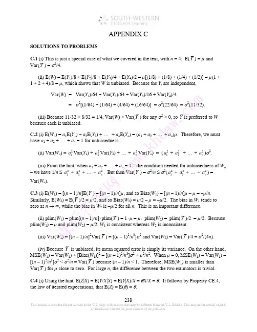
2.10(iii) From (2.57), Var(1ˆβ) = σ2/21()n i i x x =⎛⎫- ⎪⎝⎭∑. 由提示：： 21n ii x =∑ ≥ 21()n i i x x =-∑, and so Var(1β) ≤ Var(1ˆβ). A more direct way to see this is to write(一个更直接的方式看到这是编写) 21()ni i x x =-∑ = 221()n i i x n x =-∑, which is less than21n i i x=∑unless x = 0.(iv)给定的c 2i x 但随着x 的增加， 1ˆβ的方差与Var(1β)的相关性也增加.0β小时1β的偏差也小.因此, 在均方误差的基础上不管我们选择0β还是1β要取决于0β,x ,和n 的大小 (除了 21n i i x=∑的大小).3.7We can use Table 3.2. By definition, 2β > 0, and by assumption, Corr(x 1,x 2) < 0. Therefore, there is a negative bias in 1β: E(1β) < 1β. This means that, on average across different random samples, the simpleregression estimator underestimates the effect of the training program. It is even possible that E(1β) isnegative even though 1β > 0. 我们可以使用表3.2。

根据定义，> 0，由假设，科尔（X1，X2）<0。

因此，有一个负偏压为：E （）<。

这意味着，平均在不同的随机抽样，简单的回归估计低估的培训计划的效果。

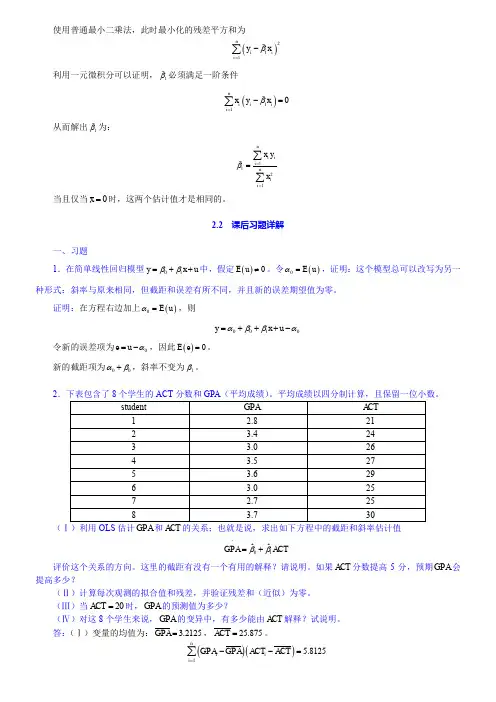
name: <unnamed>log: /Users/wangjianying/Desktop/Chapter 4 Computer exercise.smcl log type: smclopened on: 25 Oct 2016, 22:20:411. do "/var/folders/qt/0wzmrhfd3rb93j2h5hhtcwqr0000gn/T//SD19456.000000"2. ****************************Chapter 4***********************************3. **C14. use "/Users/wangjianying/Documents/data of wooldridge/stata/VOTE1.DTA"5. desContains data from /Users/wangjianying/Documents/data of wooldridge/stata/VOTE1.DTA obs: 173vars: 10 25 Jun 1999 14:07size: 4,498storage display valuevariable name type format label variable labelstate str2 %9s state postal codedistrict byte %3.0f congressional districtdemocA byte %3.2f =1 if A is democratvoteA byte %5.2f percent vote for AexpendA float %8.2f camp. expends. by A, $1000sexpendB float %8.2f camp. expends. by B, $1000sprtystrA byte %5.2f % vote for presidentlexpendA float %9.0g log(expendA)lexpendB float %9.0g log(expendB)shareA float %5.2f 100*(expendA/(expendA+expendB)) Sorted by:6. reg voteA lexpendA lexpendB prtystrASource SS df MS Number of obs = 173F( 3, 169) = 215.23 Model 38405.1096 3 12801.7032 Prob > F = 0.0000Residual 10052.1389 169 59.480112 R-squared = 0.7926Adj R-squared = 0.7889 Total 48457.2486 172 281.728189 Root MSE = 7.7123voteA Coef. Std. Err. t P>|t| [95% Conf. Interval] lexpendA 6.083316 .38215 15.92 0.000 5.328914 6.837719 lexpendB -6.615417 .3788203 -17.46 0.000 -7.363246 -5.867588 prtystrA .1519574 .0620181 2.45 0.015 .0295274 .2743873 _cons 45.07893 3.926305 11.48 0.000 37.32801 52.829857. gen cha=lexpendB-lexpendA // variable cha is a new variable//8. reg voteA lexpendA cha prtystrASource SS df MS Number of obs = 173F( 3, 169) = 215.23 Model 38405.1097 3 12801.7032 Prob > F = 0.0000Residual 10052.1388 169 59.4801115 R-squared = 0.7926Adj R-squared = 0.7889 Total 48457.2486 172 281.728189 Root MSE = 7.7123 voteA Coef. Std. Err. t P>|t| [95% Conf. Interval]lexpendA -.532101 .5330858 -1.00 0.320 -1.584466 .5202638cha -6.615417 .3788203 -17.46 0.000 -7.363246 -5.867588prtystrA .1519574 .0620181 2.45 0.015 .0295274 .2743873_cons 45.07893 3.926305 11.48 0.000 37.32801 52.829859. clear10.11. **C312. use "/Users/wangjianying/Documents/data of wooldridge/stata/hprice1.dta"13. desContains data from /Users/wangjianying/Documents/data of wooldridge/stata/hprice1.dta obs: 88vars: 10 17 Mar 2002 12:21size: 2,816storage display valuevariable name type format label variable labelprice float %9.0g house price, $1000sassess float %9.0g assessed value, $1000sbdrms byte %9.0g number of bdrmslotsize float %9.0g size of lot in square feetsqrft int %9.0g size of house in square feetcolonial byte %9.0g =1 if home is colonial stylelprice float %9.0g log(price)lassess float %9.0g log(assessllotsize float %9.0g log(lotsize)lsqrft float %9.0g log(sqrft)Sorted by:14. reg lprice sqrft bdrmsSource SS df MS Number of obs = 88F( 2, 85) = 60.73 Model 4.71671468 2 2.35835734 Prob > F = 0.0000Residual 3.30088884 85 .038833986 R-squared = 0.5883Adj R-squared = 0.5786 Total 8.01760352 87 .092156362 Root MSE = .19706 lprice Coef. Std. Err. t P>|t| [95% Conf. Interval]sqrft .0003794 .0000432 8.78 0.000 .0002935 .0004654bdrms .0288844 .0296433 0.97 0.333 -.0300543 .0878232_cons 4.766027 .0970445 49.11 0.000 4.573077 4.95897815. gen cha=sqrft-150*bdrms16. reg lprice cha bdrmsSource SS df MS Number of obs = 88F( 2, 85) = 60.73 Model 4.71671468 2 2.35835734 Prob > F = 0.0000Residual 3.30088884 85 .038833986 R-squared = 0.5883Adj R-squared = 0.5786 Total 8.01760352 87 .092156362 Root MSE = .19706lprice Coef. Std. Err. t P>|t| [95% Conf. Interval] cha .0003794 .0000432 8.78 0.000 .0002935 .0004654 bdrms .0858013 .0267675 3.21 0.002 .0325804 .1390223 _cons 4.766027 .0970445 49.11 0.000 4.573077 4.95897817. clear18.19. **C520. use "/Users/wangjianying/Documents/data of wooldridge/stata/MLB1.DTA"21. desContains data from /Users/wangjianying/Documents/data of wooldridge/stata/MLB1.DTA obs: 353vars: 47 16 Sep 1996 15:53size: 45,537storage display valuevariable name type format label variable labelsalary float %9.0g 1993 season salaryteamsal float %10.0f team payrollnl byte %9.0g =1 if national leagueyears byte %9.0g years in major leaguesgames int %9.0g career games playedatbats int %9.0g career at batsruns int %9.0g career runs scoredhits int %9.0g career hitsdoubles int %9.0g career doublestriples int %9.0g career tripleshruns int %9.0g career home runsrbis int %9.0g career runs batted inbavg float %9.0g career batting averagebb int %9.0g career walksso int %9.0g career strike outssbases int %9.0g career stolen basesfldperc int %9.0g career fielding percfrstbase byte %9.0g = 1 if first basescndbase byte %9.0g =1 if second baseshrtstop byte %9.0g =1 if shortstopthrdbase byte %9.0g =1 if third baseoutfield byte %9.0g =1 if outfieldcatcher byte %9.0g =1 if catcheryrsallst byte %9.0g years as all-starhispan byte %9.0g =1 if hispanicblack byte %9.0g =1 if blackwhitepop float %9.0g white pop. in cityblackpop float %9.0g black pop. in cityhisppop float %9.0g hispanic pop. in citypcinc int %9.0g city per capita incomegamesyr float %9.0g games per year in leaguehrunsyr float %9.0g home runs per yearatbatsyr float %9.0g at bats per yearallstar float %9.0g perc. of years an all-starslugavg float %9.0g career slugging averagerbisyr float %9.0g rbis per yearsbasesyr float %9.0g stolen bases per yearrunsyr float %9.0g runs scored per yearpercwhte float %9.0g percent white in citypercblck float %9.0g percent black in cityperchisp float %9.0g percent hispanic in cityblckpb float %9.0g black*percblckhispph float %9.0g hispan*perchispwhtepw float %9.0g white*percwhteblckph float %9.0g black*perchisphisppb float %9.0g hispan*percblcklsalary float %9.0g log(salary)Sorted by:22. reg lsalary years gamesyr bavg hrunsyrSource SS df MS Number of obs = 353F( 4, 348) = 145.24 Model 307.800674 4 76.9501684 Prob > F = 0.0000 Residual 184.374861 348 .52981282 R-squared = 0.6254Adj R-squared = 0.6211 Total 492.175535 352 1.39822595 Root MSE = .72788lsalary Coef. Std. Err. t P>|t| [95% Conf. Interval] years .0677325 .0121128 5.59 0.000 .0439089 .091556 gamesyr .0157595 .0015636 10.08 0.000 .0126841 .0188348 bavg .0014185 .0010658 1.33 0.184 -.0006776 .0035147 hrunsyr .0359434 .0072408 4.96 0.000 .0217021 .0501847 _cons 11.02091 .2657191 41.48 0.000 10.49829 11.5435323. reg lsalary years gamesyr bavg hrunsyr runsyr fldperc sbasesyrSource SS df MS Number of obs = 353F( 7, 345) = 87.25 Model 314.510478 7 44.9300682 Prob > F = 0.0000 Residual 177.665058 345 .514971181 R-squared = 0.6390Adj R-squared = 0.6317 Total 492.175535 352 1.39822595 Root MSE = .71761lsalary Coef. Std. Err. t P>|t| [95% Conf. Interval] years .0699848 .0119756 5.84 0.000 .0464305 .0935391 gamesyr .0078995 .0026775 2.95 0.003 .0026333 .0131657 bavg .0005296 .0011038 0.48 0.632 -.0016414 .0027007 hrunsyr .0232106 .0086392 2.69 0.008 .0062185 .0402027 runsyr .0173922 .0050641 3.43 0.001 .0074318 .0273525 fldperc .0010351 .0020046 0.52 0.606 -.0029077 .0049778 sbasesyr -.0064191 .0051842 -1.24 0.216 -.0166157 .0037775 _cons 10.40827 2.003255 5.20 0.000 6.468139 14.348424. test bavg fldperc sbasesyr( 1) bavg = 0( 2) fldperc = 0( 3) sbasesyr = 0F( 3, 345) = 0.69Prob > F = 0.561725. clear26. **C727. use "/Users/wangjianying/Documents/data of wooldridge/stata/twoyear.dta"28. sum phsrankVariable Obs Mean Std. Dev. Min Maxphsrank 6763 56.15703 24.27296 0 9929. reg lwage jc totcoll exper phsrankSource SS df MS Number of obs = 6763F( 4, 6758) = 483.85 Model 358.050568 4 89.5126419 Prob > F = 0.0000 Residual 1250.24552 6758 .185002297 R-squared = 0.2226Adj R-squared = 0.2222 Total 1608.29609 6762 .237843255 Root MSE = .43012 lwage Coef. Std. Err. t P>|t| [95% Conf. Interval] jc -.0093108 .0069693 -1.34 0.182 -.0229728 .0043512 totcoll .0754756 .0025588 29.50 0.000 .0704595 .0804918 exper .0049396 .0001575 31.36 0.000 .0046308 .0052483 phsrank .0003032 .0002389 1.27 0.204 -.0001651 .0007716 _cons 1.458747 .0236211 61.76 0.000 1.412442 1.50505230. reg lwage jc univ exper idSource SS df MS Number of obs = 6763F( 4, 6758) = 483.42 Model 357.807307 4 89.4518268 Prob > F = 0.0000 Residual 1250.48879 6758 .185038293 R-squared = 0.2225Adj R-squared = 0.2220 Total 1608.29609 6762 .237843255 Root MSE = .43016 lwage Coef. Std. Err. t P>|t| [95% Conf. Interval]jc .0666633 .0068294 9.76 0.000 .0532754 .0800511univ .0768813 .0023089 33.30 0.000 .0723552 .0814074exper .0049456 .0001575 31.40 0.000 .0046368 .0052543id 1.14e-07 2.09e-07 0.54 0.587 -2.97e-07 5.24e-07_cons 1.467533 .0228306 64.28 0.000 1.422778 1.51228831. reg lwage jc totcoll exper idSource SS df MS Number of obs = 6763F( 4, 6758) = 483.42 Model 357.807307 4 89.4518267 Prob > F = 0.0000Residual 1250.48879 6758 .185038293 R-squared = 0.2225Adj R-squared = 0.2220 Total 1608.29609 6762 .237843255 Root MSE = .43016 lwage Coef. Std. Err. t P>|t| [95% Conf. Interval]jc -.010218 .0069366 -1.47 0.141 -.023816 .00338totcoll .0768813 .0023089 33.30 0.000 .0723552 .0814074exper .0049456 .0001575 31.40 0.000 .0046368 .0052543id 1.14e-07 2.09e-07 0.54 0.587 -2.97e-07 5.24e-07_cons 1.467533 .0228306 64.28 0.000 1.422778 1.51228832. clear33. **C934. use "/Users/wangjianying/Documents/data of wooldridge/stata/discrim.dta"35. desContains data from /Users/wangjianying/Documents/data of wooldridge/stata/discrim.dta obs: 410vars: 37 8 Jan 2002 22:26size: 47,150storage display valuevariable name type format label variable labelpsoda float %9.0g price of medium soda, 1st wavepfries float %9.0g price of small fries, 1st wavepentree float %9.0g price entree (burger or chicken), 1st wave wagest float %9.0g starting wage, 1st wavenmgrs float %9.0g number of managers, 1st wavenregs byte %9.0g number of registers, 1st wavehrsopen float %9.0g hours open, 1st waveemp float %9.0g number of employees, 1st wavepsoda2 float %9.0g price of medium soday, 2nd wavepfries2 float %9.0g price of small fries, 2nd wavepentree2 float %9.0g price entree, 2nd wavewagest2 float %9.0g starting wage, 2nd wavenmgrs2 float %9.0g number of managers, 2nd wavenregs2 byte %9.0g number of registers, 2nd wavehrsopen2 float %9.0g hours open, 2nd waveemp2 float %9.0g number of employees, 2nd wavecompown byte %9.0g =1 if company ownedchain byte %9.0g BK = 1, KFC = 2, Roy Rogers = 3, Wendy's = 4 density float %9.0g population density, towncrmrte float %9.0g crime rate, townstate byte %9.0g NJ = 1, PA = 2prpblck float %9.0g proportion black, zipcodeprppov float %9.0g proportion in poverty, zipcodeprpncar float %9.0g proportion no car, zipcodehseval float %9.0g median housing value, zipcodenstores byte %9.0g number of stores, zipcodeincome float %9.0g median family income, zipcodecounty byte %9.0g county labellpsoda float %9.0g log(psoda)lpfries float %9.0g log(pfries)lhseval float %9.0g log(hseval)lincome float %9.0g log(income)ldensity float %9.0g log(density)NJ byte %9.0g =1 for New JerseyBK byte %9.0g =1 if Burger KingKFC byte %9.0g =1 if Kentucky Fried ChickenRR byte %9.0g =1 if Roy RogersSorted by:36. reg lpsoda prpblck lincome prppovSource SS df MS Number of obs = 401F( 3, 397) = 12.60 Model .250340622 3 .083446874 Prob > F = 0.0000Residual 2.62840943 397 .006620679 R-squared = 0.0870Adj R-squared = 0.0801 Total 2.87875005 400 .007196875 Root MSE = .08137 lpsoda Coef. Std. Err. t P>|t| [95% Conf. Interval]prpblck .0728072 .0306756 2.37 0.018 .0125003 .1331141lincome .1369553 .0267554 5.12 0.000 .0843552 .1895553prppov .38036 .1327903 2.86 0.004 .1192999 .6414201_cons -1.463333 .2937111 -4.98 0.000 -2.040756 -.885909237. corr lincome prppov(obs=409)lincome prppovlincome 1.0000prppov -0.8385 1.000038. reg lpsoda prpblck lincome prppov lhsevalSource SS df MS Number of obs = 401F( 4, 396) = 22.31 Model .529488085 4 .132372021 Prob > F = 0.0000 Residual 2.34926197 396 .00593248 R-squared = 0.1839Adj R-squared = 0.1757 Total 2.87875005 400 .007196875 Root MSE = .07702lpsoda Coef. Std. Err. t P>|t| [95% Conf. Interval] prpblck .0975502 .0292607 3.33 0.001 .0400244 .155076 lincome -.0529904 .0375261 -1.41 0.159 -.1267657 .0207848 prppov .0521229 .1344992 0.39 0.699 -.2122989 .3165447 lhseval .1213056 .0176841 6.86 0.000 .0865392 .1560721 _cons -.8415149 .2924318 -2.88 0.004 -1.416428 -.266601939. test lincome prppov( 1) lincome = 0( 2) prppov = 0F( 2, 396) = 3.52Prob > F = 0.030440.end of do-file41. log closename: <unnamed>log: /Users/wangjianying/Desktop/Chapter 4 Computer exercise.smcl log type: smclclosed on: 25 Oct 2016, 22:21:04。

ncq？0孵' 1档编制存计量经济学（第四版）习题参考答案潘省初第一章绪论试列出计量经济分析的主要步骤。

一般说来，计量经济分析按照以下步骤进行：（1）陈述理论（或假说）（2）建立计量经济模型（3）收集数据 （4）估计参数（5）假设检验（6）预测和政策分析计量经济模型中为何要包括扰动项为了使模型更现实，我们有必要在模型中引进扰动项u 来代表所有影响因变量的其它因 素，这些因素包括相对而言不重要因而未被引入模型的变量，以及纯粹的随机因素。

什么是时间序列和横截面数据试举例说明二者的区别。

时间序列数据是按时间周期（即按固定的时间间隔）收集的数据，如年度或季度的国民 生产总值、就业、货币供给、财政赤字或某人一生中每年的收入都是时间序列的例子。

横截面数据是在同一时点收集的不同个体（如个人、公司、国家等）的数据。

如人 口普查数据、世界各国2000年国民生产总值、全班学生计量经济学成绩等都是横截面 数据的例子。

估计量和估计值有何区别 估计量是指一个公式或方法，它告诉人们怎样用手中样本所提供的信息去估计总体参数。

在一项应用中，依据估计量算出的一个具体的数值，称为估计值。

如「就是一个估 n 计量，F = J 。

现有一样本，共4个数，100, 104, 96, 130,则根据这个样本的数据 n第二章 计量经济分析的统计学基础略，参考教材。

请用例中的数据求北京男生平均身高的99%置信区间运用均值估计量得出的均值估计值为100 + 104 + 96 +130 =107.5 oS _5用二，N-l=15个自由度查表得%105f 故99%置信限为± Z0.0055.V =174±X = 174±也就是说，根据样本，我们有99%的把握说，北京男高中生的平均身高在至厘米之间。

25个雇员的随机样本的平均周薪为130元，试问此样本是否取自一个均值为120元、标准差为10元的正态总体原假设“o：〃 = 12O备择假设”1：〃工120检验统计量查表Z0.o25 =1% 因为Z=5>Z O.025 = 1.96,故拒绝原假设，即此样本不是取自一个均值为120元、标准差为10元的正态总体。