连续系统与离散系统的互转(s域与z域互转)
- 格式:pdf
- 大小:182.64 KB
- 文档页数:4
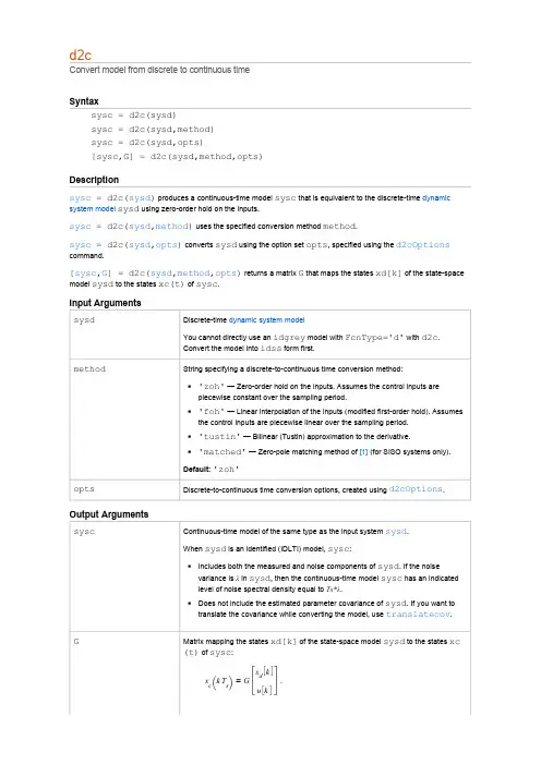
Convert model from discrete to continuous timed2cSyntaxsysc = d2c(sysd)sysc = d2c(sysd,method)sysc = d2c(sysd,opts)[sysc,G] = d2c(sysd,method,opts)Descriptionsysc = d2c(sysd) produces a continuous-time model sysc that is equivalent to the discrete-time dynamic system model sysd using zero-order hold on the inputs.sysc = d2c(sysd,method) uses the specified conversion method method.sysc = d2c(sysd,opts) converts sysd using the option set opts, specified using the d2cOptions command.[sysc,G] = d2c(sysd,method,opts) returns a matrix G that maps the states xd[k] of the state-space model sysd to the states xc(t) of sysc.Input Argumentssysd Discrete-time dynamic system modelYou cannot directly use an idgrey model with FcnType='d' with d2c.Convert the model into idss form first.method String specifying a discrete-to-continuous time conversion method:◾'zoh' — Zero-order hold on the inputs. Assumes the control inputs arepiecewise constant over the sampling period.◾'foh' — Linear interpolation of the inputs (modified first-order hold). Assumesthe control inputs are piecewise linear over the sampling period.◾'tustin' — Bilinear (Tustin) approximation to the derivative.◾'matched' — Zero-pole matching method of [1] (for SISO systems only).Default: 'zoh'opts Discrete-to-continuous time conversion options, created using d2cOptions. Output Argumentssysc Continuous-time model of the same type as the input system sysd.When sysd is an identified (IDLTI) model, sysc:◾Includes both the measured and noise components of sysd. If the noisevariance is λ in sysd, then the continuous-time model sysc has an indicatedlevel of noise spectral density equal to Ts*λ.◾Does not include the estimated parameter covariance of sysd. If you want totranslate the covariance while converting the model, use translatecov.G Matrix mapping the states xd[k] of the state-space model sysd to the states xc(t) of sysc:x c (k Ts)=G24xd[k]u[k]35.Given an initial condition x0 for sysd and an initial input u0 = u[0], thecorresponding initial condition for sysc (assuming u[k] = 0 for k< 0 is givenby:ExamplesExample 1Consider the following discrete-time transfer function:Suppose the model has sample time T s = 0.1 s. You can derive a continuous-time zero-order-hold equivalent model with the following commands:H = tf([1 -1], [1 1 0.3], 0.1);Hc = d2c(H)Hc =121.7 s + 3.026e-12---------------------s^2 + 12.04 s + 776.7Continuous-time transfer function.Discretizing the resulting model Hc with the default zero-order hold method and sampling time T s = 0.1s returns the original discrete model H (z ):c2d(Hc,0.1)ans =z - 1-------------z^2 + z + 0.3Sample time: 0.1 secondsDiscrete-time transfer function.To use the Tustin approximation instead of zero-order hold, typeHc = d2c(H,'tustin');As with zero-order hold, the inverse discretization operationc2d(Hc,0.1,'tustin');gives back the original H (z ).Example 2Convert an identified transfer function and compare its performance against a directly estimated continuous-time model.load iddata1sys1d = tfest(z1,2,'Ts',0.1);x c (0)=G 24x 0u 035.H (z )=z −1z 2+z +0.3sys1c = d2c(sys1d,'zoh');sys2c = tfest(z1,2);compare(z1,sys1c,sys2c)The two systems are virtually identical.Example 3Analyze the effect of parameter uncertainty on frequency response across d2c operation on an identified model.load iddata1sysd = tfest(z1, 2, 'Ts', 0.1);sysc = d2c(sysd, 'zoh');sys1c has no covariance information. Regenerate it using a zero iteration update with the same estimation command and estimation data:opt = tfestOptions;opt.SearchOption.MaxIter = 0;sys1c = tfest(z1, sysc, opt);h = bodeplot(sysd, sysc);showConfidence(h)The uncertainties of sysc and sysd are comparable up to the Nyquist frequency. However, sysc exhibits large uncertainty in the frequency range for which the estimation data does not provide any information.If you do not have access to the estimation data, use translatecov which is a Gauss-approximation formula based translation of covariance across model type conversion operations.LimitationsThe Tustin approximation is not defined for systems with poles at z = –1 and is ill-conditioned for systems with poles near z = –1.expand allThe zero-order hold method cannot handle systems with poles at z = 0. In addition, the 'zoh' conversion increases the model order for systems with negative real poles, [2]. The model order increases because the matrix logarithm maps real negative poles to complex poles. Single complex poles are not physically meaningful because of their complex time response.Instead, to ensure that all complex poles of the continuous model come in conjugate pairs, d2c replaces negative real poles z = –α with a pair of complex conjugate poles near –α. The conversion then yields a continuous model with higher order. For example, to convert the discrete-time transfer functiontype:Ts = 0.1 % sample time 0.1 sH = zpk(-0.2,-0.5,1,Ts) * tf(1,[1 1 0.4],Ts)Hc = d2c(H)These commands produce the following result.Warning: System order was increased to handle real negative poles.Zero/pole/gain:-33.6556 (s-6.273) (s^2 + 28.29s + 1041)--------------------------------------------(s^2 + 9.163s + 637.3) (s^2 + 13.86s + 1035)To convert Hc back to discrete time, type:c2d(Hc,Ts)yieldingZero/pole/gain:(z+0.5) (z+0.2)-------------------------(z+0.5)^2 (z^2 + z + 0.4)Sampling time: 0.1This discrete model coincides with H (z ) after canceling the pole/zero pair at z = –0.5.More AboutTipsAlgorithms References[1] Franklin, G.F., Powell,D.J., and Workman, M.L., Digital Control of Dynamic Systems (3rd Edition), Prentice Hall, 1997..[2] Kollár, I., G.F. Franklin, and R. Pintelon, "On the Equivalence of z-domain and s-domain Models in SystemIdentification," Proceedings of the IEEE ® Instrumentation and Measurement Technology Conference, Brussels, Belgium, June, 1996, Vol. 1, pp. 14-19.See Alsoc2d | d2cOptions | d2d | logm | translatecov H (z )=z +0.2(z +0.5)(z 2+z +0.4)。