Monte Carlo Simulations of Star Clusters
- 格式:pdf
- 大小:112.55 KB
- 文档页数:6

蒙特卡罗法简单介绍和案例蒙特卡罗法历史悠久。
1773年法国G.-L.L.von 布丰曾通过随机投针试验来确定圆周率π的近似值,这就是应用这个方法的最早例子。
蒙特卡罗是摩纳哥著名赌城,1945年 J.von 诺伊曼等人用它来命名此法,沿用至今。
数字计算机的发展为大规模的随机试验提供了有效工具,遂使蒙特卡罗法得到广泛应用。
在连续系统和离散事件系统的仿真中,通常构造一个和系统特性相近似的概率模型,并对它进行随机试验,因此蒙特卡罗法也是系统仿真方法之一。
对于蒙特卡罗技术应用于不可预见费的估算的研究,是对蒙特卡罗技术应用的拓展,能更好地了解尝试其在项目管理方面更多的应用,用其解决项目管理的问题。
用蒙特卡罗技术研究不可预见费,尝试用蒙特卡罗解决一般项目的不可预见费求取问题,避免不可预见费过高过低的问题。
蒙特卡洛方法的基本思想是:将符合一定概率分布的大量随机数作为参数带入数学模型,求出所关注变量的概率分布,从而了解不同参数对目标变量的综合影响以及目标变量最终结果的统计特性。
蒙特卡洛方法的基本原理简单描述如下:假定函数),...,,(21nx x x f y =,蒙特卡洛方法利用一个随机数发生器通过抽样取出每一组随机变量 (ni i i x x x ,...,,21),然后按),...,,(21n x x x f y =的关系式确定函数的值),...,,(21ni i i i x x x f y =。
反复独立抽样(模拟)多次(i=1,2,…),便可得到函数的一组抽样数据(n y y y ,...,,21),当模拟次数足够多时,便可给出与实际情况相近的函数y 的概率分布与其数字特征。
蒙特卡罗法(Monte Carlo Simulation )也称随机模拟,它主要依据概率分布对随机变量进行抽样,然后将样本带入数学模型进行计算得到应变量。
虽然蒙特卡罗模拟技术只给出的是统计估计而非精确的结果且应用其研究问题需要花费大量的计算时间,但它对问题的维数不敏感,对求解对象是线性问题与否也没有原则性要求,因此在复杂系统的不确定分析中,蒙特卡罗方法成为不可或缺的手段。


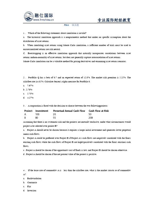
FRM一级真题1 . Which of the following statements about simulation is invalid?a. The historical simulation approach is a nonparametric method that makes no specific assumption about the distribution of asset returns.b. When simulating asset returns using Monte Carlo simulation, a sufficient number of trials must be used to ensuresimulated returns are risk neutral.C. Bootstrapping is an effective simulation approach that naturally incorporates correlations between asset returns andnon-normality of asset returns, but does not generally capture autocorrelation of asset returns.Monte Carlo simulation can be a valuable method for pricing derivatives and examining asset return scenarios.2 . Portfolio Q has a beta of 0.7 and an expected return of 12.8%. The market risk premium is 5.25%. The risk-free rate is4.85%. Calculate Jensen's Alpha measure for Portfolio 0.a. 7.67%b . 2.70%c. 5.73%d. 4.27%3 . A corporation is faced with the decision to choose between the two followingproiects:Assuminq that there is no svstematic risk and the proiects are mutuallv exclusive, under what circumstances would project A be selected over proiect B?a. Project A should never be chosen because it requires a larqer initial investment and qenerates lower perpetual annua cash flows.b. Project A could be preferred over Project B if Project A's cash flows are neqativelv correlated with the firm's existinq cash flows while the cash flows of Project B are hiqhlvpositivelv correlated with the firm's existinci cash flows.c . Project A should be chosen if the opportunitv cost of funds is low, and Project B should be chosen otherwise.d . Project A should be chosen if the net present value of the proiect is positive.4 . If the lease rate of commoditv A is less than the risk-free rate, what is the market structu re of commoditv A?a. Backwardationb. Contancioc. Flatd. Inversion5 . Sarah is a risk manacier responsible for the fixed income portfolio of a larqe insurance companv. The portfolio contains a 30-vear zero coupon bond issued bv the US Treasurv (STRIPS) with a 5% vield. What is the bond's DV01 ?a. 0.0161b. 0.0665c. 0.0692d. 0.0694。


蒙特卡洛模拟风险分析是我们制定的每个决策的一部分。
我们一直面对着不确定,不明确和变异。
甚至我们无法获得信息,我们不能准确的预测未来。
蒙特卡洛模拟( Monte Carlo simulation)让您看到了您决策的所有可能的输出,并评估风险,允许在不确定的情况下制定更好的决策。
什么是蒙特卡洛模拟( Monte Carlo simulation)蒙特卡洛模拟( Monte Carlo simulation)是一种计算机数学技术,允许人们在定量分析和决策制定过程中量化风险。
这项技术被专家们用于各种不同的领域,比如财经,项目管理,能源,生产,工程,研究和开发,保险,石油&天然气,物流和环境。
蒙特卡洛模拟( Monte Carlo simulation)提供给了决策制定者大范围的可能输出和任意行动选择将会发生的概率。
它显示了极端的可能性-最的输出,最保守的输出-以及对于中间路线决策的最可能的结果。
这项技术首先被从事原子弹工作的科学家使用;它被命名为蒙特卡洛,摩纳哥有名的娱乐旅游胜地。
它是在二战的时候被传入的,蒙特卡洛模拟( Monte Carlo simulation)现在已经被用于建模各种物理和概念系统。
蒙特卡洛模拟( Monte Carlo simulation)是如何工作的蒙特卡洛模拟( Monte Carlo simulation)通过构建可能结果的模型-通过替换任意存在固有不确定性的因子的一定范围的值(概率分布)-来执行风险分析。
它一次又一次的计算结果,每次使用一个从概率分布获得的不同随机数集。
根据不确定数和为他们制定的范围,蒙特卡洛模拟( Monte Carlo simulation)能够在它完成计算前调用成千上万次的重复计算。
蒙特卡洛模拟( Monte Carlo simulation)产生可能结果输出值的分布。
通过使用概率分布,变量能够拥有不同结果发生的不同概率。
概率分布是一种用来描述风险分析的变量中的不确定性的更加可行的方法。
a r X i v:h e p -l a t /9312002v 1 1 D e c 19931Monte Carlo Simulations of the SU(2)Vacuum StructureA.R.Levia ∗aCenter for Theoretical Physics,Laboratory for Nuclear Science and Department of Physics,Massachusetts Institute of Technology,Cambridge,Massachusetts 02139U.S.A.and Department of Physics,Boston University,590Commonwealth Ave.,Boston,Massachusetts 02215U.S.A.Lattice Monte Carlo simulations are performed for the SU(2)Yang Mills gauge theory in the presence of an Abelian background with external sources to obtain information on the effective potential.The goal is to investigate the lowest Landau mode that,in the continuum one-loop effective potential,is the crucial mode for instability.It is shown that also in the lattice formulation this lowest Landau mode plays a very peculiar role,and it is important for the understanding of the vacuum properties.1.INTRODUCTIONTo understand the IR behavior of non-Abelian gauge theory a non-perturbative framework is necessary.Therefore,lattice formulation is par-ticularly useful.However,the comparison be-tween one-loop perturbative expansion and lat-tice regularization might give important informa-tion.From this comparison we can learn about the trustworthiness of perturbative expansion.Furthermore,the loop expansion can provide in-dicative information for the lattice quantities.Despite the importance of Yang-Mills theories,the complete solution of non-Abelian gauge the-ories has yet to be found.In order to gain a bet-ter understanding of these theories,a necessary first step is the study of their vacuum structures.Nevertheless,the vacuum structure of such theo-ries has yet to be understood even in the simplest case,i.e.SU(2)without matter.Moreover,the infrared properties of such theories must be stud-ied systematically if we want to have some clue on confinement.Many authors have studied one-loop effective potential for SU(2)and the possible consequences [1,2].In addition,several Monte Carlo simula-tions have already been done with a wild range of techniques in 3and 4Dimensions[2,3].2Hδb 3(xδµ2−yδµ1).(2)2With this choice,the well known Savvidy result for the one-loop effective potential is obtainedE(H)=H248π2 ln gH2−i6πν(4)whereνare the eigenvalues of the second deriva-tive of the action with respect to the gaugefields, and the summation is over all the eigenvalues. This expression is a natural consequence of the saddle point approximation:V(H)=V classic−¯hδηδη+O(¯h2)(5)whereΩis the volume factor.The eigenvalue of this problem can be found by realizing that there is the same symmetry as the one of the Lan-dau levels problem,therefore we have exactly the same class of solutions.That yield to the eigen-valuesν=k2+(2n+1+2S z)gH(6) where k=k20+k2z,n=0,1,2,...and S z=±1is the gluon polarization.For the lowest landau mode,i.e.n=0,S z=−1,we haveν<0that give the imaginary part of the effective potential.Note that with Abelian background it is possible to obtain all eigenvalues positive only by insertion of non-gauge invariant terms in the TTICE RESULTSUntil now we have argued that this lowest Lan-dau mode plays a very particular role on the one loop perturbative expansion.This motivated us to understand what happened to this mode on lattice where the task is non-perturbative.To extract information on this mode on lattice we noted that,due to thefiniteness of the lat-tice k z,is quantized as well,with k z=2mπ/L z, where m is an integer.Therefore,the lowest in-homogeneous z-mode,m=1,becomes stable for lattices the extent of which in the z-direction is smaller thanL criticz=2πgH.(7)This enables us to search for the critical sizeL criticz.The homogeneous mode,m=0,which is always unstable,is eliminated by imposing a delta condition in the path integral.We perform Monte Carlo simulations that gen-erate a backgroundfield H in the z direction in the presence of an Abelian source of strength j. We use a heat bath updating procedure with periodic boundary conditions and for the com-putational technique we address to reference[2]. To eliminate the homogeneous mode m=0we force the Polyakov line in the z direction to take a fixed value different from zero.Monte Carlo sim-ulations are made with a lattice volume L3∗L z, where L is the size of the x,y,t directions.The finite effect due to L is not so crucial.In fact,for the observable that we are interested,it is suffi-cient to use L=12−16.Simulations are made by varying L z from4to50.The expectation value of the plaquette in the 1-2plane P[F12]as a function ofβand j is mea-sured.We monitor the quantityX=P[F12(β,0)]−P[F12(β,j)]3interested,these other contributions are smoothly variable functions,and thus they will not affect the critical behavior.We evaluated X for different values of βand j performing,for large j 4500sweeps after dis-charging 500for thermalization.For smaller j we increase the number of sweeps until a significant amount of datawas collected.Our data [2]show that there is no sign of the unstable mode away from the critical βregion (β=2.1−2.5).The situation changes dramat-ically in the critical region where the instability appears as a decrease of the vacuum energy con-tribution to the plaquette in the z direction.This effect becomes more evident in the presence of strong sources.The fact that the instability dis-appears outside of the scaling window is a strong evidence that the instability is a distinguishing feature of the continuum rather than the strong coupling vacuum.In order to study the IR prop-erty of the continuum theory we should remain in the region where the instability is manifest.The disappearance of the instability as β→0may give a clue to understanding the difference between the physics of the continuum and the strong coupling lattice theory.We systematically analyzed the critical region of βfor several values of j .The values of L critic z(β,j )are obtained by interpolating the kink of X and taking the median value.L critic zwas found to be dependent on the source j and on βin this region according to the renormal-ization group dependence.It is clear from our data that L critic zbelongs to the confinement phase and that there is good agreement with the renor-malization group equation.Our data follow the same dependence of the deconfinament transition [6]as should be for a dimensional scale length.Hence the ratio between the L critic and the de-confinament scale parameter L dec is independent of β.The relevant physical quantities must be obtained in the limit of vanishing of the induced field Q (j )→0.From our data we obtain L critic zL critic z (m )=T decm .(10)The simulations show that these modes followwith good approximation eq.(10).This is strong evidence for the harmonicity of this modes.This is a quite surprising result because we are in a re-gion of strong non-perturbative effects.It is stim-ulating to think in terms of a parallel between the situation described above and the integer Quan-tum Hall Effect.This similarity is based on the dual picture (z ↔t ,E ↔H ,etc...),and on the plateau structures for each mode.AcknowledgementsIt is a pleasure to thank Janos Polonyi and Suzhou Huang for several useful discussions.REFERENCES1.G.K.Savvidy,Phys.Lett.71B (1977)133;S.G.Matinyan and G.K.Savvidy Nucl.Phys.B134(1978)539;N.K.Nielsen and P.Olesen,Nucl.Phys.B144(1978)376;H.B.Nielsen and M.Ninomiya Nucl.Phys.B156(1979)1;J.Ambjørn and P.Olesen,Nucl.Phys.B170(1980)60and 265;J.Ambjørn,B.Felsager and P.Olesen,Nucl.Phys.B175(1980)349;L.Maiani,G.Martinelli,G.C.Rossi and M.Testa,Nucl.Phys.B273(1986)275.2. A.R.Levi and J.Polonyi,preprint CTP 2161.3.J.Ambjørn et al,Phys.Lett.245B (1990)575;P.Cea and L.Cosmai,Phys.Lett.249B (1990)114,264B (1991)415;Phys.Rev.D43(1991)620;preprint BARI-TH 129/93;H.D.Trot-tier and R.M.Woloshyn,Phys.Rev.Lett.70(1993)2053.4.L.F.Abbott,Nucl.Phys.B185(1981)189,and references therein.5.S.Huang and A.R.Levi,preprint BU-HEP-93-22.6.J.Kuti,J.Polonyi and K.Szlachanyi,Phys.Lett.98B (1981)199;E.Kovacs,Phys.Lett.118B (1982)125.。
实验四受限空间中的高分子链穿越纳米管道的Monte Carlo模拟一、实验目的1.了解键涨落算法(BFM)的基本原理;2.观察受限空间中的高分子链穿越纳米管道的动力学过程;二、实验原理结构是材料物理性能的物质基础。
不同的物质其结构不同,性能当然也不同。
但是性能常常必须通过分子运动才能表现出来。
因此,我们必须深切了解分子运动特点,才能建立高分子的结构和性能的内在联系。
另一方面,生物体系的研究表明,为了实现和完成细胞功能,蛋白质分子经常必须要穿越水和膜物质形成的界面,例如一些特殊的RNA 分子在复制和传递遗传信息时穿越细胞核膜的过程,DNA分子从病毒注射进入寄主细胞,基因在细菌之间的转换以及抗菌素感染等等。
因此,大分子穿越纳米孔(管道)的动力学过程对于生命体系来说是极其重要也是非常普遍的。
同时,类似的穿越过程有着很广泛而又重要的科技应用前景,例如DNA组成序列的分析,长链DNA在凝胶电泳中的分离。
因此,研究高分子链的穿越机制具有十分重要的理论及实际意义。
高分子链穿越纳米管道的动力学行为是极其复杂的过程,受到各种因素的影响,例如分子链的柔性,驱动力的大小,链单元之间以及与管壁的相互作用。
由于实验对各种实验条件和参数的控制比较困难,对所取得的结果的分析和理解也有很大的局限性。
此时,计算机模拟在大分子穿越纳米管道的动力学之一研究领域发挥着极其重要的作用。
Monte Carlo方法在数学上称其为随机模拟(random simulation)方法,随机抽样(random sampling)技术或统计实验(statistical testing)方法。
它的基本思想是:为了求解数学、物理、几何、化学等问题,建立一个概率模型或随机过程,使它的参数等于问题的解;当所解的问题本身属随机性问题时,则可采用直接模拟法,即根据实际物理情况的概率法来构造Monte Carlo模型;然后通过对模型,或过程的观察,或抽样实验来计算所求参数的统计特征,最后给出所求解的近似值。
/share/detail/5568877蒙特卡罗(Monte Carlo)方法,或称计算机随机模拟方法,是一种基于“随机数”的计算方法。
这一方法源于美国在第一次世界大战进研制原子弹的“曼哈顿计划”。
该计划的主持人之一、数学家冯·诺伊曼用驰名世界的赌城—摩纳哥的Monte Carlo—来命名这种方法,为它蒙上了一层神秘色彩。
Monte Carlo方法的基本思想很早以前就被人们所发现和利用。
早在17世纪,人们就知道用事件发生的“频率”来决定事件的“概率”。
19世纪人们用投针试验的方法来决定圆周率π。
本世纪40年代电子计算机的出现,特别是近年来高速电子计算机的出现,使得用数学方法在计算机上大量、快速地模拟这样的试验成为可能。
考虑平面上的一个边长为1的正方形及其内部的一个形状不规则的“图形”,如何求出这个“图形”的面积呢?Monte Carlo方法是这样一种“随机化”的方法:向该正方形“随机地”投掷N个点落于“图形”内,则该“图形”的面积近似为M/N。
可用民意测验来作一个不严格的比喻。
民意测验的人不是征询每一个登记选民的意见,而是通过对选民进行小规模的抽样调查来确定可能的优胜者。
其基本思想是一样的。
科技计算中的问题比这要复杂得多。
比如金融衍生产品(期权、期货、掉期等)的定价及交易风险估算,问题的维数(即变量的个数)可能高达数百甚至数千。
对这类问题,难度随维数的增加呈指数增长,这就是所谓的“维数的灾难”(Course Dimensionality),传统的数值方法难以对付(即使使用速度最快的计算机)。
Monte Carlo方法能很好地用来对付维数的灾难,因为该方法的计算复杂性不再依赖于维数。
以前那些本来是无法计算的问题现在也能够计算量。
为提高方法的效率,科学家们提出了许多所谓的“方差缩减”技巧。
另一类形式与Monte Carlo方法相似,但理论基础不同的方法—“拟蒙特卡罗方法”(Quasi-Monte Carlo方法)—近年来也获得迅速发展。
ACCA P4考试:Monte Carlo Simulation本文由高顿ACCA整理发布,转载请注明出处Traditional sensitivity analysis can be used if one project variable changes independently of all others. However, some project variables may be interdependent (e.g. production volume and unit costs).Simulation is a technique which allows more than one variable to change at the same time. The classic example of simulation is the "Monte Carlo" method which can be used to estimate not only a project's NPV but also its volatility.Designing a Monte Carlo SimulationAn assessment of the volatility (or standard deviation) of the net present value of a project requires estimates of the distributions of the key input parameters and an assessment of the correlations between variables. Some of variables may be normally distributed (e.g. demand), but others may be assumed to have limit values and a most likely value (e.g. redundancy costs).In its simplest form, Monte Carlo simulation assumes that the input variables are uncorrelated. More sophisticated modelling can, however, incorporate estimates of the correlation between variables.Monte Carlo simulation then employs random numbers to select a specimen value for each variable in order to estimate a "trial value" for the project NPV. This is repeated a large number of times until a distribution of net present values emerges. This distribution will approximate a normal distribution.Refinements such as the Latin Hypercube technique can reduce the likelihood of spurious results occurring through chance in the random number generation process.Outputs From Monte Carlo SimulationThe output from the simulation will give the expected NPV for the project and a range of other statistics including the standard deviation of the output distribution.In addition, the model can rank the significance of each variable in determining the project NPV.Summary of Monte Carlo Simulation1. Specify the major variables.2. Specify the relationship between the variables.3. Attach probability distributions (e.g. the normal distribution) to each variable and assign random numbers to reflect the distribution.4. Simulate the environment by generating random numbers.5. Record the outcome of each simulation.6. Repeat simulation many times to obtain a frequency distribution of the NPV.7. Determine the expected NPV and its standard deviation.更多ACCA资讯请关注高顿ACCA官网:。
a rXiv:as tr o-ph/6438v13J un2Dynamics of Star Clusters and the Milky WayASP Conference Series,Vol.000,2000S.Deiters,B.Fuchs,A.Just,R.Spurzem,and R.Wielen,eds.Monte Carlo Simulations of Star Clusters Mirek Giersz Nicolaus Copernicus Astronomical Center,Polish Academy of Sciences,ul.Bartycka 18,00-716Warsaw,Poland Abstract.A revision of Stod´o l kiewicz’s Monte Carlo code is used to simulate evolution of large star clusters.The survey on the evolution of multi–mass N –body systems influenced by the tidal field of a parent galaxy and by stellar evolution is discussed.For the first time,the sim-ulation on the ”star–by–star”bases of evolution of 1,000,000body star cluster is presented.1.Introduction Very detailed,recent observations of globular clusters suggest very close in-terplay between stellar evolution,binary evolution and dynamical interactions.This interplay is far from being understood.Monte Carlo codes,which use a sta-tistical method of solving the Fokker–Planck equation provide all the necessary flexibility to disentangle the mutual interaction between physical processes im-portant during globular cluster evolution.The codes were developed by Spitzer (1975,and references therein)and H´e non (1975,and references therein)in the early seventies,and substantially improved by Marchant &Shapiro (1980,and references therein)and Stod´o l kiewicz (1986,and references therein)and recently reintroduced by Giersz (1998,2000),Heggie et al.1999,Joshi et al.(1999a),Joshi et al.(1999b,hereafter JNR)and Rasio (2000,this volume).The Monte Carlo scheme takes full advantage of the undisputed physical knowledge of the secular evolution of (spherical)star clusters as inferred from continuum modelsimulations.Additionally,it describes in a proper way the graininess of the grav-itational field and the stochasticity of the real N –body systems and provides as detailed as in direct N –body simulations information about movement of any objects in the system.This does not include any additional physical approxima-tions or assumptions which are common in Fokker–Planck and gas models (for e.g.conductivity).Because of this,the Monte Carlo scheme can be regarded as a method which lies between direct N –body and Fokker–Planck models and combines most of their advantages.Moreover,Monte Carlo codes are simple,very fast,easily parallelized and easily scalable to the physical units.There is no need for special hardware or supercomputers to efficiently simulate evolu-tion of realistic star clusters .However,as any numerical method,the Monte Carlo method suffers from some disadvantages.It can only deal with spherically symmetrical systems,and only small–angle two–body interactions.The galac-tic tidal field can only be approximated by the tidal cut-off,and unfortunately,cross–sections for some physical processes are needed (e.g.three–body binary12M.Gierszformation).Additionally,the physical processes,which evolve on time–scales comparable to the crossing time–scale,can not be properly investigated,and the method has difficulty with the proper definition of local parameters(e.g. density,velocity dispersion).Despite all of these disadvantages the Monte Carlo method can be easily and efficiently used to simulate evolution of realistic glob-ular clusters.The comparison between numerical simulations and observations will help to infer the initial parameters of proto–clusters and help to disentangle the interplay between physical processes involved in cluster evolution.More-over,the Monte Carlo method can be used to simulate dynamical formation of massive black holes in dense spherical stellar systems(e.g.galactic nuclei).2.ResultsThe Monte Carlo code is described in detail in Giersz(1998),which deals with simulations of isolated single–mass systems.Here and in Giersz(2000)the Monte Carlo code is extended to include the following additional physical processes:•multi–mass systems described by the power–law initial mass function:N(m)dm=Cm−αdm,m min≤m≤m max,where C andαare con-stants.•stellar evolution introduced according to prescription given by Chernoff& Weinberg(1990,hereafter CW)or Taut et al.(1997).•three–body binaries described by the suitably modified Spitzer’s formula (Spitzer1987,Giersz2000).•binary–binary interactions introduced according to Mikkola(1983,1984) and Stod´o l kiewicz(1986).•tidalfield simulated by tidal cut-offwith energy and/or apocenter criterion.The results of Monte Carlo simulations of star cluster evolution will be presented in the next two subsections.2.1.Family∼1The initial conditions were chosen in a similar way as in a collaborative ex-periment(Heggie et al.1999).The positions and velocities of all stars were drawn from a King model.All standard models have the same total mass M=60000M⊙and the same tidal radius R c=30pc.Masses are drawn from the power–law mass function described above.The minimum mass was chosen as0.1M⊙and maximum mass as15M⊙.Three different values of the power–law index were adopted:α=1.5,2.35and3.5.The set of initial King models was characterized by W0=3,5and7.Additional models of CW’s Family1were computed to facilitate comparison with results of other simulations(minimum mass equal to0.4M⊙,α=1.5,2.5,3.5and total mass M=90685M⊙,99100M⊙, 103040M⊙,respectively).In Table1the comparison between available results of N-body,Fokker–Planck and Monte Carlo simulations is presented.The standard models show a remarkably good agreement with N-body results(Heggie2000).See columnsMonte Carlo Simulations of Star Clusters3 labeled by G and H-0.1in Table1.Only models with aflat mass function show some disagreement.These models are difficult for both methods.Violent stellar evolution and induced strong tidal striping lead to troubles with time–scaling for the N-body model and proper determination of the tidal radius for the Monte Carlo model.Generally,the same is true for Monte Carlo models of Family1. Results of these models show good agreement with results of CW,Aarseth& Heggie(1998)and Takahashi&Portegies Zwart(1999).JNR’s results,particu-larly for strongly concentrated systems,disagree with all other models.This can be connected with the fact,that JNR’s Monte Carlo scheme is not particularly suitable for high central density and strong density contrast.Too large deflec-tion angles adopted by JNR and consequently too large time-steps can lead to too fast evolution in these models.Table1.Time of cluster collapse or disruption aCW JNR H-0.1G-0.40.28 5.211.30.7W33532.0>20.017.6--0.50.07 W5235/25-13.5 6.8-- 6.026.1 W715b 3.1 1.2 2.19.6 3.0 1.79.8W7359.99.20.74M.Gierszand in consequence to different evolution of the total mass,anisotropy,etc.. Models which are quickly disrupted show only small signs of mass segregation. Models with larger central concentration survive the phase of rapid mass loss and then undergo core collapse and subsequent post–collapse expansion in a manner similar to isolated models.The expansion phase is eventually reversed when tidal limitation becomes important.As in isolated models,mass segregation substantially slows down by the end of the core collapse.After a core bounce there is a substantial increase in the mean mass in the middle and outer parts of the system,caused by the preferential escape of stars of low mass and tidal effects.Standard models,which are not quickly disrupted,show modest initial build up of anisotropy in the outer parts of the system.As the tidal stripping exposes inner parts of the system,anisotropy gradually decreases and eventually becomes slightly negative.The central part of the system stays nearly isotropic. Models of Family1,from the very beginning,develop in the outer parts of the system modest negative anisotropy.It stays negative until the time of cluster disruption,when it becomes slightly positive(during cluster disruption most stars are on radial orbits).2.2.1,000,000body runFor thefirst time,the Monte Carlo simulation,on the”star–by–star”bases, of evolution of1,000,000body star cluster is presented.The initial conditions were as follows:total mass equal to319,305M⊙,tidal radius equal to33.57pc, power–low index of mass function equal to−2.35,minimum and maximum mass equal to0.1M⊙and15.0M⊙,respectively and King model parameter W0=5.The1,000,000body run shows basically the same features as,discussed above,models of Family∼1.As an example of the overall cluster evolution the time dependence of Lagrangian radii,core radius and tidal radius are presented in Figure1.The three different phases of evolution can be clearly distinguished. First,short phase of violent mass loss due to stellar evolution leads to overall cluster expansion.Even the innermost Lagrangian radius expands,the con-traction connected with mass segregation is not strong enough to dominate the expansion.Second phase is characterized by the slow core collapse.Tidal effects are small and cluster behaves in a similar way as an ordinary isolated system. Then in the third phase,post–collapse evolution is superposed with growing tidal striping effects.The cluster nearly homogeneously contracts.The central parts of the system show clear signs of the gravothermal oscillations.In Figure2the density profiles for the different epochs are presented.It is clear,that in the central parts of the system the density profile shows steeper slope than−2.2(line labeled by6),the standard value for single–mass systems. This is in agreement with results of CW.The power–low index is a function of the ratio of mass of the most massive stars to the average mass.The larger the ratio the smaller the power–law index.The core is mainly populated by the most massive stars(massive white dwarfs,neutron stars and black holes), whose masses are larger than the average mass in the vicinity of the core.So as a consequence,the power–law index is smaller than−2.2.The density profiles for an advanced collapse phase(lines labeled by4,5and6)show a bump in the middle part of the system(close to0.08in x–axis).The bump originates because of the growing influence of low mass stars on the determination of theMonte Carlo Simulations of Star Clusters 50.0010.010.1110050001000015000200002500030000L o g (r )Time (Myr)M = 319,305 MoN = 1,000,000Wo = 5Rtide = 33.57 pcalpha = -2.350.5%Mmin = 0.1 Mo Mmax = 15.0 Mo Rc 10%50%99%RtideFigure 1.Evolution of the Lagrangian radii,core radius and tidal radius,labeled by 0.5%,10%,50%,99%,Rc and Rtide,respectively.0.00010.0010.010.11101001000100000.0010.010.1110l o g (ρ)log(r)M = 319,305 Mo N = 1,000,000Mmin = 0.1 Mo Mmax = 15.0 Mo alpha = -2.35Rtid = 33.57 pcWo = 51 - 0 Myr2 - 2 Myr3 - 10 Myr4 - 13 Myr5 - 14.5 Myr6 - 15.1 Myr 213456-2.2Figure 2.Density profiles for the different epochs (labels from 1to 6on the figure).The straight line indicates the power–law with exponent -2.2.6M.Gierszlocal density.The position and the size of the bump is in a good agreement with Fokker–Planck results(Takahashi&Lee2000).In order to perform simulations of real globular clusters several additional physical effects have to be included into the code.The tidal shock heating of the cluster due to passages through the Galactic disk,interaction with the bulge,shock–induced relaxation,primordial binaries,physical collisions between single stars and binaries are one of them.Inclusion of all these processes do not pose a fundamental theoretical or technical challenge.It will allow to perform detailed comparison between simulations and observed properties of globular clusters and will help to understand the globular cluster formation conditions and explain how peculiar objects observed in clusters can be formed.These kinds of simulations will also help to introduce,in a proper way,into future N–body simulations all necessary processes to simulate on the star–by–star basis evolution of real globular clusters from their birth to death.Acknowledgments.I would like to thank Douglas C.Heggie for making the N–body results of standard model simulations available.ReferencesAarseth S.L.&Heggie D.C.,1998,MNRAS,297,794ChernoffD.F.&Weinberg M.D.,1990,(CW),ApJ,351,121Giersz M.,1998,MNRAS,298,1239Giersz M.,2000,MNRAS,submittedHeggie D.C.,2000,private informationHeggie D.C.,Giersz M.,Spurzem R.,Takakashi K.,1999,in Highlights of As-tronomy,vol11,ed.J.Andersen,591H´e non M.,1975,in Hayli A.,ed.,Dynamics of Stellar Systems,Reidel:Dor-drecht,133Joshi K.,J.,Nave C.&Rasio F.A.,1999a,ApJ submitted(astro-ph/9912155) Joshi K.,J.,Rasio F.A.&Portegies Zwart S.,1999b,(JNR),ApJ submitted (astro-ph/9909115)Marchant A.B.&Shapiro S.L.,1980,ApJ,239,685Mikkola S.,1983,MNRAS,205,733Mikkola S.,1984,MNRAS,208,75Rasio F.A.,2000,in Spurzem R.,et al.,eds,Dynamics of Star Clusters and the Milky Way,(ASP Conference Series)Spitzer L.,Jr.,1975,in Hayli A.,ed,Dynamics of Stellar Systems,Reidel: Dordrecht,p.3Spitzer L.,Jr.,1987,Dynamical Evolution of Globular Clusters.Princeton Univ.Press,Princeton,77Stod´o l kiewicz J.S.,1986,Acta Astr.,36,19Takahashi K.&Lee H.M.,1999,MNRAS submitted(astro-ph/9909006) Takahashi K.&Portegies Zwart,S.F.,1999,ApJ submitted(astro-ph/9903366) Tout C.A,Aarseth S.J.,Pols O.R.&Eggleton P.P,1997,MNRAS,291,732。