Thaden A Simulation Framework for Schema-based Query Routing

SolidWorks Simulation图解应用教程（一）发表时间： 2009-11-10 来源: e-works关键字: SolidWorks Simulation CosmosWorks SolidWorks2009SolidWorks Simulation作为SolidWorks COSMOSWorks的新名称，是与SolidWorks完全集成的设计分析系统。

它提供了单一屏幕解决方案来进行应力分析、频率分析、扭曲分析、热分析和优化分析，凭借着快速解算器的强有力支持，使用户能够使用个人计算机快速解决大型问题。

SolidWorks Simulation提供了多种捆绑包，可满足各项分析需要。

为什么要分析?在我们完成了产品的建模工作之后，需要确保模型能够在现场有效地发挥作用。

如果缺乏分析工具，则只能通过昂贵且耗时的产品开发周期来完成这一任务。

一般产品开发周期通常包括以下步骤：1)建造产品模型;2)生成设计的原型;3)现场测试原型;4)评估现场测试的结果;5)根据现场测试结果修改设计。

这一过程将一直继续、反复，直到获得满意的解决方案为止。

而分析可以帮助我们完成以下任务：1)在计算机上模拟模型的测试过程来代替昂贵的现场测试，从而降低费用;2)通过减少产品开发周期次数来缩短产品上市时间;3)快速测试许多概念和情形，然后做出最终决定。

这样，我们就有更多的时间考虑新的设计，从而快速改进产品。

SolidWorks Simulation作为SolidWorks COSMOSWorks的新名称，是与SolidWorks完全集成的设计分析系统。

它提供了单一屏幕解决方案来进行应力分析、频率分析、扭曲分析、热分析和优化分析，凭借着快速解算器的强有力支持，使用户能够使用个人计算机快速解决大型问题。

SolidWorks Simulation提供了多种捆绑包，可满足各项分析需要。

为了使读者能更详尽地了解SolidWorks Simulation的分析应用功能，从本期开始，我们将分期介绍其强大的分析功能。

英语论文范文精选篇一Chapter OneINTRODUCTION1.1 Research BackgroundHigh proficiency in writing is a key to success in a wide variety of situations andprofessions; meanwhile it is of critical importance for students to apply for promising jobs.Writing skills for university students are among the overwhelming indicators of success inacademic work during their freshmen year of college (Geiser & Studley, 2001). Writingskills for professionals are critical for their daily work and essential for application andpromotion within their disciplines (Light, 2008). Writing induces the capability ofconstructing logics, articulating ideas, debating opinions, and sharpening multipleperspectives. As a result, effective writing is conducive to associating convincingly withcommunication targets, including teachers, peers, colleagues, coworkers, and thecommunity at large (Crowhurst, 1990). No wonder that writing skill is an indispensible partto be checked for every test at home and abroad，such as TOELF, lELTS，GRE, BEC，CET4, CET6, TEM4，TEM8 and so on.Notwithstanding such manifestation of the significance of writing, it is reported in the2002 National Assessment of Educational Progress (NAEP) report in the U.S.A. that lessthan a third of students in Grade 4 (28%)，Grade 8 (31%), and Grade 12 (21%) scored at orabove proficient levels，and only 2% wrote at advanced levels for all three samples.Moreover, only 9% of Grade 12 Black students and only 28% of Grade 12 White studentswere able to write at a proficient level (National Center for Educational Statistics, 2003).……………1.2 Significance of the ResearchBased on the CET 4 and CET6 compositions extracted from the CLEC，the study aimsto reveal the relationship between the linguistic features and the writing quality by meansof the advanced software，namely Lexical Frequency Profile, Coh-Metrix3.0 and L2Syntactic Complexity Analyzer for the analysis of vocabulary, syntax and textual cohesion.This study will be of great value mainly for the following two aspects:Firstly, theoretically speaking, the study is going to offer guidance and reference forthe teachingmethodology of L2 writing. The study reveals the contribution of lexicaldiversity, syntactic complexity, textual cohesion to writing quality, reflects the mostdecisive factor of the writing quality and analyzes the mutual relationship between thelexical diversity and quality of writing, the syntactic complexity and quality of writing aswell as the textual cohesion and quality of writing. Hopefully, this research will shedsome light on the instruction of CET 4 and 6 writing and provide practical advice.Secondly, practically speaking, the study demonstrates a new direction for thedevelopment of automatic assessment of the writing. The study is to be carried out bothby means of software and labor work to comprehensively examine more than 28variables that might have an impact on writing quality and build the relation modelbetween these related variables and writing scores. ……………Chapter TwoLITERATURE REVIEW2.1 Lexical Features and Quality of WritingIn the process of L2 writing，students are always perplexed by vocabulary. Leki&Carson (1994) surveyed 128 L2 learners to know about their feelings on the courseEnglish for Academic Purposes (EAP). It is discovered that the strongest zeal for studentsis to improve their language proficiency, especially lexical proficiency. Jordan (1997)obtained the similar conclusion in his study on Chinese students in UK applying for theirmaster degrees, 62% of whom regarded vocabulary as their biggest problem in the processof English writing. Over the past two decades，researchers have attached more and more importance toL2vocabulary studies. As an important element of language proficiency, lexical proficiency isdefined from different perspectives and evaluated by a series of measurements. Meanwhile, lexical proficiency, to a large extent, is embodied by lexical features. As a matter of fact,studies on lexical features have received more and more attention from home and abroadresearchers mainly focusing on total words, lexical diversity (LD) or lexical richness (LR)and lexical complexity (LC), among which lexical diversity or lexical richness has gainedmore popularity for lexical proficiency study.……………2.2 Syntactic Features and Quality of WritingSyntactic complexity (also called syntactic maturity，or linguistic complexity)，isimportant in the prediction of the quality of student writings. Wolfe-Quintero et al. (1998)pointed out that a syntactically complex writer uses a wide variety of both basic andsophisticated structures，while a syntactically simple writer uses only a narrow range ofbasic structures. In the past half century, researchers adopted many different indices tostudy the syntactic complexity and attempted to find out the relationship among the scores,the grades, the ages and the writing quality. Syntactic complexity is defined as “the range of forms that surface in languageproduction and the degree of sophistication of such forms” (Ortega, 2003). It is animportant factor in the second language assessment construct as described in Bachman's(1990) conceptual model of language ability, and therefore is often used as an index oflanguage proficiency and development status of L2 learners. Various studies have proposedand investigated measures of syntactic complexity as well as examined itspredictivenessfor language proficiency, in both L2 writing and speaking settings, which will be reviewedrespectively.Syntactic complexity is also called syntactic maturity, referring to the range oflanguage production form and the degree of the form complexity. Therefore，the length ofthe production unit, the amount of the sentence embeddedness and the range of thestructure type are all the subjects of the syntactic complexity (Ortega 2003: 492).………CHAPTER THREE METHODOLOGY (20)3.1 Composition Collection (20)3.2 Tools (21)3.3 Variables (23)3.3.1 Dependent variables (25)3.3.2 Independent variables (26)3.4 Data Analysis (28)CHAPTER FOUR DATA ANALYSIS AND RESULTS (30)4.1 Quantitative Differences in High- and Low- Proficiency Writings-1ivviv (30)4.2 Comparison between Quantitative Features of CET4 (38)4.3 Impacts of Quantitative Features on Writing Quality (47)5.1 Lexical Diversity and Writing Quality (47)5.2 Syntactic Complexity and Writing Quality (48)5.3 Textual Cohesion and Writing Quality (49)Chapter FiveDICUSSION5.1 Lexical Diversity and Writing QualityU index assessing lexical diversity has showed significant difference between high-and low-proficiency writing both in CET4 and CET6. It may suggest thathigh-proficiencywritings have displayed more diverse vocabularies, which is different from the study ofWang (2004). In his study, the target students have a similar lexical diversity. Among theindices assessing lexical study in his study, none index has showed significant differencebetween high- and low-proficiency writings or correlated with writings scores. In his study,he explained the possible reason for such a result that there issignificant difference inaverage words. However, this result is probably attributed to his measurement of lexicaldiversity. In his study, TTR was employed as an index of lexical diversity, but asmentioned above, TTR is reliable only when texts have the same length. In Wang's study,texts vary in length; thus longer texts tend to have lower TTR. That is why the relationshipbetween lexical diversity and writing quality is blurred. But in this study, we adopted Uindex to measure lexical diversity in CET compositions, for U index can avoid theweakness of TTR and eliminate the influence of text length. Besides, Liu (2003) studied 57second- year college students in two natural classes and found out that vocabulary size hadno immediate effect on writing score. However, the result that lexical diversity has apositive impact on the quality of writing in this study is in accordance with the study ofMcNamara et al. (2001).……………ConclusionThis study aims to explore the relationship between lexical features and L2 writingquality with the help of Lexical Frequency Profile, the relationship between syntacticfeatures and L2 writing quality through the use of the computational tool L2 SyntacticComplexity Analyzer and the relationship between cohesive features and second languagewriting quality with the help of the computational tool Coh-Metrix3.0. Meanwhile, thestudy gives us information about the textual representation of different writingproficiencies along multiple textual measurements.This section summarizes the major findings of this study and presents theoretical,methodological and pedagogical implications for L2 writing research. Limitation of thepresent study and suggestions for further studies are raised in the end.……………Reference (omitted)英语论文范文精选篇二Chapter One Introduction1.1 Background of the ResearchEnglish writing is an important way of communication, which can enhance the ability oflanguage acquisition in the process of second language learning. As one of the language skills,English writing is very difficult to master. After many years, students still find that their writingis unsatisfactory and have many problems. It is widely acknowledged that much attentionshould be paid to English writing. At present our college English writing teaching is time-consuming and low effectiveness, for teachers spend a lot of time and energy reading andcorrecting students’ compositions, but the efficiency is not high; at the same time, studentsspend a lot of time writing, and the results are not satisfactory.The following conspicuous problems tend to exist in the English writing. First, when givena topic, students tend to think in Chinese and do a translation job. Second, students spend toomuch time avoiding grammatical errors in the process of writing, which leads to the ignoranceof the organization of the compositions in a comprehensive view. Third, enriching the contentduring the writing process is difficult for students, for they fail to support their viewpointswithappropriate examples and strong arguments. English writing is the weakest part in Englishlearning especially for Chinese Vocational college students. According to Basic Teaching Requirements for Vocational College English Course,developing students’ comprehensi ve abilities to use English language is the teaching aim ofvocational college English. In terms of writing, students should have the ability to master thebasic writing skills and accomplishing writing tasks of different types, including narration,description, argumentation and practical writings like business email or announcement.Besides,their writing should have a clear organization and proper coherence; at the same time, studentsshould be able to write or describe something with adequate content and proper form indifferent situations, such as business situation.…………1.2 Purpose and Significance of the ResearchAs we can see, most English class in the vocational colleges is always a big class which contains at least sixty students and in the class students may not receive the feedbackfromteacher immediately, although offering feedback is one of the essential tasks. It is helpful andefficient for teachers that students themselves can check other s’ writing and give comments. Sothese two feedbacks have their own roles in the revision. Considering the vocational collegeeducation, examining the practice of teacher feedback and peer feedback on EFL writing is ofgreat importance and necessity. This study is aimed to discuss the effects of teacher feedbackand peer feedback in the English class in order to provide some useful English writing teachingmethod and studying ways for vocational college education. This is not only consistent with thespirit of the new curriculum; at the same time reflects the “student-c entered” teachingphilosophy.…………Chapter Two Literature Review2.1 Feedback TheoryFeedback is widely seen in education as crucial for both encouraging and consolidatinglearning (Anderson, 1982; Brophy, 1981; Vygotsky, 1978), and the importance has alsobeenacknowledged in the field of English writing.In language learning, feedback means evaluative remarks which are available to languagelearners concerning their language proficiency or linguistic performance(Larsen-Freeman,2005). In the filed of teaching and learning, feedback is defined as many terms, such asresponse, review, correction, evaluation or comment. No matter what the term is, it can bedefined as “comments or information learners receive on the success of a learning task, eitherfrom the teacher or from other learners (Richards et al., 1998)”.A more detailed description of feedback in terms of writing is that the feedback is “inputfrom a reader to a writer with the effect of providing information to the writer for revision”(Keh, 1990). From the presentation of general grammatical explanation to the specific errorcorrection is all the range of feedback. The purpose is to improve the writing ability of studentsby the description and correction of the errors.The role of feedback is to make writers learn where he or she has misled or confused thereader by supplying insufficient information, illogical organization, lack ofdevelopment ofideas, or something like inappropriate word-choice or tense (Keh, 1990).…………2.2 Theoretical Foundations of FeedbackCollaborative learning, also called cooperative learning, is the second theoretical basis thatback for the application of feedback in writing class. It is feasible that students communicateactively with each other in the classroom.There is a clear difference betweenstudents-centered and traditional teacher-ledclassrooms. Students’ enthusiasm of participating in group discussion strengthens whenstudents are completely absorbed in collaborative learning in the students-centered class. Whenstudents get together to work out a problem, ideas are conveyed among them and immediatefeedback is received from their group members.Collaborative learning emphasizes that both students and instructors participate and interact actively (Hiltz, 1997). Collaborative learning is viewed from both behavioral andhumanistic perspectives (Slavin 1987). The behavioral perspective stresses that students areencouraged to study under a cooperativesituation and rewarded in the form of group rather thanindividual ones. As for the humanistic perspective, more understanding and better performanceare gained from the interaction among peers. So it is obvious that collaborative learning putsmore attention to the influence of peers, which is different from the previous English writingteaching theories(Johnson and Johnson,1986).Collaborative learning make the students work and learn together to maximize their ownand other’s study.…………Chapter Three Research Methodology (21)3.1 Research Questions (21)3.2 Subjects (21)3.3 Instruments (22)3.3.1 Writing Tasks (23)3.3.2 Questionnaires (23)3.3.3 Pre-test and Post-test (24)3.4 Research Design (24)3.5 Data Collection (27)Chapter Four Results Presentation and Discussion (29)4.1 Students’ Changed Writing P roficiency (29)4.2 Students’ Changed Interest in English Learning and Writing (36)Chapter Five Conclusion (43)5.1 Major Findings (43)5.2 Pedagogical Implications and Suggestions (44)5.3 Limitations of the Study (46)5.4 Suggestions for Further Study (46)Chapter Four Results Presentation and Discussion4.1 Students’ Changed Writing ProficiencyThe data from the pre-test and post-test of the EC and CC were all collected and analyzedthrough SPSS 13.0 to investigate the difference before and after the adoption of teacherfeedback and peer feedback in the English writing class. As table4-1 shows, the mean score of the control class (11.43) is rather similar to theexperimental class (11.56). Moreover, the standard deviation of experimental class (9.357) isalso rather similar to that of the control class (9.421). The mean score of the experimental groupisa little bit higher than that of control the group(11.56>11.43), but the disparity is only 0.13,and thelowest score and the highest score of the two groups are quite close to each other.On the basis of the group statistics of the pre-test, the author carried out an independentsamples t-test in order to further compare the mean scores of the pre-test between CC and EC.Table 4-2 shows the Sig is 0.624, higher than 0.05, showing the writing proficiency of twogroups have no significant difference. Thereby, the statistics in the row of “Equal variancesassumed” should be observed. The Mean Difference is merely 0.338, and the Standard ErrorDifference is only 2.086. In addition, Sig. (2-tailed) is 0.836 (>.05), which indicates that thestudents from both EC and CC share almost the same level of English writing proficiencybefore the study.…………ConclusionFeedback plays a key role and is quite effective in enhancing students’ writingproficiency. The comparison of mean scores in pre-test and post-test indicates that both groupsof EG and CG make more progress in their writingafter this feedback-initiated writinginstruction. Teacher feedback and peer feedback can lead to achievements in students’ writing,which means that the two kinds of feedback are all helpful, effective for promoting students’writing competence to some degree and there is no definite answer for the research question,which one will enhance students’ writing ability the more effective method between teacherfeedback and peer feedback. Teacher and peer feedback play different roles in improvingstudents’ writing. When giving teacher feedback, students in the control class make greaterprogress in organization and content, which was different from the experimental class. Theresults and discussion on students’ focus on the five language aspects had been mentioned in theprevious chapter. Those deep-level language aspects, like the content and organization are theweakest points for most of the students especially for the vocational students, so teacher has theability to point out the mistakes more deeply. As for peer feedback, students may havedifficultyin recognizing the errors in those deep -level aspects so they put more attention to the grammarand vocabulary.……………Reference (omitted)英语论文范文精选篇三Chapter I Introduction1.1 Theoretically analytical tool of the thesisAiming to analyze the features of English advertisements, the author picks English1advertisements which closely relate to people's daily life and rank first on the list ofcommercial advertisements as the studying material and applies thematic structure andthematic progression patterns as the theoretical tool of analysis.Now, quite a large number of linguists have studied theme and rheme, usingthematic structure and thematic progression patterns to conduct studies on detaileddiscourses，such as novels, sports news and students' theses. Taking thematic structureand thematic progression patterns as the analytical tool can help to explore how textsare developed. Halliday，a great linguist who has made many contributions tolinguistics, claims thematic structure as "basic form ofthe organization of the clause asmessage" (Halliday 1985:34). Each clause can be divided into theme part and rhemepart. The relation between themes and rhemes of the text can reveal how the text isconducted, which is known as thematic progression. Through thematicprogression,coherence of the text can be established. …………1.2 Purpose of the studyThrough the perspective of Systemic-Functional Grammar, 42 written texts ofEnglish advertisements are taken as the corpus and their thematic structures andthematic progression patterns are analyzed one by one. The author will analyze thedistribution of different themes and explore the use of four basic thematic progressionpatterns in this type of advertisements, trying to answer three questions:(1) What are the features of the usage of different themes in English advertisements?(2) Which thematic progression is used most often and why?(3) What pragmatic effects do these four thematic progressions have in Englishadvertisements?In the whole thesis, these three questions will be answered through analyzing theparticularEnglish advertisements. Halliday's(1994) theory of thematic structure and XuShenghuan's(1982) four basic thematic progression patterns will be adopted asanalytical framework, the reason of which will be explained later in Chapter 2.…………Chapter II Literature review2.1 Studies on thematic structureTheme and rheme distinction was firstly described by V. Mathesius in 1939 (HuZhuanglin 1994:137). In his mother tongue, Czech，he tries to analyze sentences fromthe perspective of communication and function and show how the information in asentence is expressed. Firbas translates Mathesius' definition of theme as: "[the theme]is that which is known or at least obvious in the given situation and from which thespeaker proceeds."(Martin 1992:434) Therefore, according to him, theme is the startingpoint of the message, which is known or given in the utterance and from which thespeaker proceeds, while rheme plays a role as new information, which is about what thespeaker says ontheme and represents the very important information that the speakerwants to convey to the hearer. In his opinion，a clause is divided into three parts: theme,rheme and transition. Of course, it is obvious that Mathesius does not use the exactexpression of "theme" and "rheme".Though Mathesius' point of view has some deficiencies, it influences Praguescholars greatly. One of his well-known followers, Firbas, proposes a view to improvethe thematic theories. He believes that theme is one that has lower degree ofcommunicative dynamism in some certain context while rheme has higher one.Different from Mathesius in dividing a clause into three parts (Hu Zhuanglin et al1989)，Firbas (1992) merges the concept of transition into rheme and divides a clauseinto two.Following with their opinions, there are two groups differing from each other. Onegroup thinks that theme is equal to "given" while the other one, Systemic School,accepts 'separating approach' which disentangles the two. Systemic School argues thatthere are differences existing between information structure (given-new) and thematicstructure (theme-rheme).…………2.2 Studies on thematic progression patternsIn discourse analysis，a sentence is understood as a message，conveyinginformation from the speaker to the listener. It can be separated into two segments:theme and rheme. Mathesius' (1976) concept of theme and rheme leads to a surge ofinterest in discourse analysis operated at the level of clause. The different choices andorders of discourse themes, the mutual connection and hierarchy between themes andrhemes, as well as their relationship to the hyperthemes of the superior discourse (suchas the paragraph, chapter, etc.) to the whole text or to the situation would influence theinternal structure of the text. Halliday (1985:227) subscribes to that opinion too，statingthat "the success of a text does not lie in the grammatical correctness of its individualsentences，but in the multiple relationships established among them". Therefore,thematic progression performs an important role in discourse analysis.Both scholars abroad and at home make great contributions to the study ofthematic structure together with thematic progression.…………Chapter III Analytical framework of the study and research design (20)3.1 Analytical framework of the study (20)3.1.1 Analytical framework of thematic structure (21)3.1.2 Analytical framework of thematic progression patterns (22)3.2 Research design (24)3.2.1 Consideration on selecting data used in the analysis (25)3.2.2 Analytical procedures (27)3.3 Summary (30)Chapter IV Analysis of thematic structure (33)4.1 Some rules of identifying and counting themes........334.2 Simple theme, multiple theme and zero theme (35)4.2.1 Distribution of simple theme, multiple theme and zero theme (36)4.2.? Data analysis (38)4.3 Textual theme, interpersonal theme and experiential theme (39)4.3.1 Distribution of three functional themes (40)4.3.2 Data analysis (42)4.4 Summary (43)Chapter V Analysis of thematic progression patterns........445.1 Distribution of thematic progression patterns (44)5.2 Data analysis (44)5.3 Summary (45)Chapter V Analysis of thematic progression patterns5.1 Distribution of thematic progression patternsBefore discussing the distribution of thematic progression patterns, anadvertisement sample will be taken as an example, which is selected from Michelin.Example 3:GE(T1) is building the world by providing capital, expertise and infrastructure for a globaleconomy(Rl). GE Capital(T2) has provided billions in financing so businesses can build and growtheir operations and consumers can build their financial futures(R2). We(T3) build appliances,lighting, power systems and other products that help millions of homes, offices, factories and retailfacilities around theworld work better(R3).^In this example given above, themes and rhemes have already been marked forconvenience. T1 refers to the theme of the first clause while R1 refers to the rheme, andso on. These three sentences in this piece of advertisement are all concerned about GEenterprise, although there is a slight difference among them. According to ZhuYongsheng (1985)，these themes can be seen as the same one and these clauses aresharing the same theme. ……………ConclusionThis thesis is focused on the thematic structure and thematic progression patternsof English advertisements, aiming to find some features and favored patterns.A literature review on thematic structure，thematic progression patterns andEnglish advertisements is made before the detailed analysis and finds that fewresearches are done on advertisements with a perspective of thematic organization andby a case study of one specific kind of advertisements. Therefore, the author conducts astudy on English advertisements by setting a theoretical framework,including theHalliday's theory of thematic structure and Xu Shenghuan's classification of thematicprogression patterns. Through these methods，the research is done by investigating thestatistics and results are given below: English advertisements prefer to use simpler themes to convey' informationquickly and directly. Multiple themes and clauses with themes omitted are used not sooften and differ from each other not so much in number because of the uniquecharacteristics of advertisements.……………Reference (omitted)英语论文范文精选篇四第一章引言1.1研究背景传统的课堂英语教学已经不能满足日益提高的英语学习要求，而网络化的英语在线学习系统提供大量不断更新的资源，突破地域和时间的限制，为学生和教师提供课内或课外的网络学习平台。

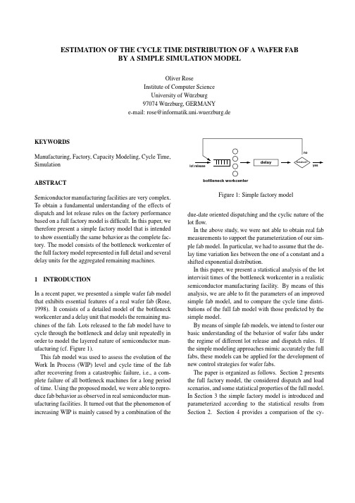
ESTIMATION OF THE CYCLE TIME DISTRIBUTION OF A W AFER FAB BY A SIMPLE SIMULATION MODELOliver RoseInstitute of Computer ScienceUniversity of W¨u rzburg97074W¨u rzburg,GERMANYe-mail:rose@informatik.uni-wuerzburg.deKEYWORDSManufacturing,Factory,Capacity Modeling,Cycle Time, SimulationABSTRACTSemiconductor manufacturing facilities are very complex. To obtain a fundamental understanding of the effects of dispatch and lot release rules on the factory performance based on a full factory model is difficult.In this paper,we therefore present a simple factory model that is intended to show essentially the same behavior as the complete fac-tory.The model consists of the bottleneck workcenter of the full factory model represented in full detail and several delay units for the aggregated remaining machines.1INTRODUCTIONIn a recent paper,we presented a simple wafer fab model that exhibits essential features of a real wafer fab(Rose, 1998).It consists of a detailed model of the bottleneck workcenter and a delay unit that models the remaining ma-chines of the fab.Lots released to the fab model have to cycle through the bottleneck and delay unit repeatedly in order to model the layered nature of semiconductor man-ufacturing(cf.Figure1).This fab model was used to assess the evolution of the Work In Process(WIP)level and cycle time of the fab after recovering from a catastrophic failure,i.e.,a com-plete failure of all bottleneck machines for a long period of ing the proposed model,we were able to repro-duce fab behavior as observed in real semiconductor man-ufacturing facilities.It turned out that the phenomenon of increasing WIP is mainly caused by a combination of thebottleneck workcenterFigure1:Simple factory modeldue-date oriented dispatching and the cyclic nature of the lotflow.In the above study,we were not able to obtain real fab measurements to support the parameterization of our sim-ple fab model.In particular,we had to assume that the de-lay time variation lies between the one of a constant and a shifted exponential distribution.In this paper,we present a statistical analysis of the lot intervisit times of the bottleneck workcenter in a realistic semiconductor manufacturing facility.By means of this analysis,we are able tofit the parameters of an improved simple fab model,and to compare the cycle time distri-butions of the full fab model with those predicted by the simple model.By means of simple fab models,we intend to foster our basic understanding of the behavior of wafer fabs under the regime of different lot release and dispatch rules.If the simple modeling approaches mimic accurately the full fabs,these models can be applied for the development of new control strategies for wafer fabs.The paper is organized as follows.Section2presents the full factory model,the considered dispatch and load scenarios,and some statistical properties of the full model. In Section3the simple factory model is introduced and parameterized according to the statistical results from Section2.Section4provides a comparison of the cy-cle time distributions of both models for several scenarios and a discussion of the capabilities of the simple factory model.2FULL FACTORY MODELAs test fab for our experiments,we chose the slightly modified MIMAC fab#6testbed data set that we obtained from Prof.Fowler(MASMLAB,Arizona State Univer-sity,).MIMAC(Mea-surement and Improvement of MAnufacturing Capacity) was a joint project of JESSI/MST and SEMATECH to identify and measure the effects and interactions of ma-jor factors that cause loss in fab efficiency(Fowler and Robinson,1995).Fab#6consists of228machines and97operators.It manufactures9types of wafers each of which has more than10layers and requires more than250process steps. The modified fab produces no scrapped wafers and has only6products because there are3products that do not require the bottleneck workcenter for being processed. With respect to dispatch rules it should be noted that setup avoidance is always used in our experiments.The time be-tween lot starts of each product is constant.We use the Factory Explorer simulation tool to collect the following datasets from the modified MIMAC#6full fab model(Wright Williams&Kelly,1997).Given a bot-tleneck load and a dispatch rule for all workcenters/tool groups,we record for each product the following delays. We consider the time from lot start until itfirst reaches the bottleneck,the start delay,for each cycle separately the time it takes to reenter the bottleneck after leaving it, the cycle delay,and the time from leaving the bottleneck for the last time until having left the fab,thefinal delay. For each considered time period several thousand mea-surements are taken.The measured intervals consist of processing times,setup times,and waiting times.Then, for each of the data sets a theoretical distribution is se-lected.The decision is based on Q-Q-plots and sums of squared differences of the measurements’histograms and several distribution candidates.In addition,the autocorre-lation function of each dataset is computed for thefirst30 lags.We consider the following four scenarios:FIFO and CR with a bottleneck load of80%and95%,respectively.The dispatch rules are defined as follows.FIFO(First In First Out)The waiting lots are sched-uled in the order of their arrival.This rule does not lead to a reordering of queued lots.CR(Critical Ratio)Each time a lot has to be taken from the queue,the following index is assigned to each of the waiting lots:CRdue date current timeremaining processing time The lot with the smallest index value is chosen for processing.As a consequence,lots that are closer to their due dates are preferred.For a review on dispatch rules see(Wein,1988)or(Ather-ton and Atherton,1995).For each scenario the simulation is run for10years of fab time.Thefirst year’s measurements are not consid-ered to avoid initialization bias.We obtain for each time period of interest at least2000measurements.For each scenario more than100distributions have to befitted.To keep the model simple we intend to use only one class of distributions to model all delays.It turns out that the class of shifted Gamma distributions provide the best match among all tested candidates.For each shifted Gamma distribution three parameters have to be estimated:the shape parameter,the scale parame-ter,and the shift parameter.First,we determine the set of parameters that minimizes the squared distance of the empirical density of the measured data and the shifted Gamma density function.Then,while keeping the scale parameter,the two other parameters are recomputed in or-der to obtain the same mean and variance for empirical data and theoretical density function.This method offers the best result with respect to providing a good match in shape of the distributions of the delays while achieving the exact values for mean and variance.As an example, Figure2shows the empirical distribution of thefirst cy-cle delay of product1of the CR95%scenario.The other fitted gamma distributions show approximately the same level of accuracy.For the95%scenarios,almost all sequences of mea-surements show considerable correlation.In most cases, the lag-1coefficients of correlation are larger than0.5and the decays of the autocorrelation functions are slower than exponential for at least thefirst ten lags.Figure3shows the empirical autocorrelation curve for thefirst30lags of the aforementioned sequence of measurements.These correlations originate basically from the fact that subsequent lots of the same product and the same layer,0.010.020.030.040.050.06020406080100120140hoursdata gammaFigure 2:Example distribution of a cycle delay00.10.20.30.40.50.60.7051015202530lagFigure 3:Example correlations of a cycle delay i.e.,the same bottleneck intervisit cycle,see the fab and its machines in roughly the same state.Due to dispatch rules such as FIFO or CR,overtaking of lots is avoided to a large extent.In addition,lots are grouped while waiting for batch completion at batch machines such as oxidation ovens.3SIMPLE FACTORY MODELIn order to predict the cycle time distributions correctly,the model used in (Rose,1998)has to be modified.The general idea of a detailed model of the bottleneck work-center and delay units representing all other workcenters is kept.The bottleneck model includes the number of ma-chines,the processing times of each product,and the ap-plication of the full fab dispatch rule.There is one delay unit for the time spent by a lot from release to first entering the bottleneck work center,one delay unit for the period oftime that it takes from departing the bottleneck machines until reentering the bottleneck queue,and a delay unit for the time from leaving the bottleneck for the last time until finishing the final processing step.The model is depicted in Figure 4.bottleneck workcenterFigure 4:Modified simple factory modelAll delays are modeled by shifted Gamma distributions that are parameterized as mentioned in Section 2.For each product the delays are determined individually.The same holds for each product’s cycle delays.To model correlated delays,we choose the following approach.If we add two random variables that are Gamma distributed with a common shape parameter the result is Gamma distributed with the same shape parameter and a scale parameter that is the sum of the two single ones (Law and Kelton,1991).Given a sequence of random variables that are distributed for a pos-itive integer .Then,the sumis distributed for .The coefficients ofcorrelation result infor ,and for ,because we keep values and replace just a single value to compute from .This simple approach facilitates a delay model with Gamma distributed delays having a linearly decreasing correlation structure.The modeling of delays with other correlation structures,such as autoregressive processes,while still providing Gamma distributed values is consid-erably more complex than the above method (Cario and Nelson,1996).4RESULTSThe simple factory model is implemented in ARENA 3.01(Kelton et al.,1997).The duration of each run is 10years of simulated time.Measurements taken during the first year are cut off.To determine whether both the simple factory model and the full factory model exhibit the same behavior,our primary goal is to match cycle times for each product in mean,variance,and shape of distribution for both models.In the following experiments,lot release and,as a con-sequence,bottleneck loads are exactly the same for both models.We first consider FIFO dispatching.In the 80%load scenario the correlations of the delays are low compared to the 95%case.Thus,we used uncorrelated delay units for the simple fab model.Figure 5shows the cycle times of product #1.The histograms of the cycle times for the simple and the full factory models match well.The same holds for all other products.00.0020.0040.0060.0080.010.0120.0140.0160.018550600650700750800hoursfull simpleFigure 5:Product #1cycle times (FIFO 80%)In the FIFO 95%load scenario,the delays are consid-erably correlated with empirical lag-1coefficients of cor-relations ranging from about 0.5up to 0.9.To keep the model simple,we apply two correlation scenarios:mod-erate with a lag-1correlation of 0.66()and strong with a lag-1correlation of 0.9().Without model-ing the correlations the histogram shapes look similar but the mean cycle times are too low.Introducing positive correlation has a clumping effect on the lots because con-secutive lots of the same product have similar delays.It turns out,however,that this lot clumping does not result in higher cycle times as expected.Figure 6depicts the product #1cycle time histograms of the full fab and the simple fab with uncorrelated delays.The histograms for the correlated delays are not shown because they almost match the uncorrelated one.In the following,CR dispatching is considered.The FIFO dispatching at 95%load leads to an average flow factor over all products of about 2.1,where the flow fac-tor is defined as the ratio of average cycle time and raw processing time.The target flow factor for the CR 95%scenario is set to 2.1.This results in shorter cycle times for all but one product and a considerable reduction of00.0020.0040.0060.0080.010.01270075080085090095010001050hoursfull simpleFigure 6:Product #1cycle times (FIFO 95%)variance of cycle times for all products.This is a typi-cal result for switching from FIFO to CR in a wafer fab (Brown et al.,1997).In Figure 7cycle time histograms of product #1under the regime of FIFO and CR are provided.00.0050.010.0150.020.0250.030.03570075080085090095010001050hoursCR FIFOFigure 7:Product #1cycle times (FIFO/CR 95%)Figure 8shows the cycle time histograms of the CR 95%scenario.In contrast to the FIFO scenarios,the shapes of the histogram curves do not match well for ei-ther strength of correlation.This result is caused by a special property of the CR dispatch rule.The application of CR not only completely avoids overtaking of lots of the same product and cycle,such as FIFO does,but also to a large extent overtaking of lots of the same product that are in different cycles,and of lots of different products.Here,lot overtaking is defined as lots being processed earlier at the bottleneck than lots that are closer to their due date.In the full factory model this kind of overtaking only rarely happens because at each machine the lots are processed according to their due dates.In the simple model,however,this reordering0.0050.010.0150.020.0250.030.03565070075080085090095010001050hoursfull simpleFigure 8:Product #1cycle times (CR 95%)0.0050.010.0150.020.0250.030100200300400500600700800900hoursFigure 9:Full factory model histograms of cycle comple-tion timesof lots does only take place at the bottleneck workcenter.Only the effect of overtaking of lots of the same product and cycle is reduced by introducing correlation that leads to lot clumping.The variance reduction effect of CR is visualized in Fig-ure 9and Figure 10.In both cases lots have the same distribution of cycle delays for each cycle,but the shapes of histograms of the periods of time taken from lot start to finishing a particular cycle are considerably different.In case of full factory with CR,most of the histograms of consecutive cycles are clearly separated (cf.Figure 9)whereas the histograms in the case of simple factory with CR overlap (cf.Figure 10).Due to CR,lots of one product being in the same cycle are grouped together with respect to cycle times in the full factory model.Table 1shows the mean and standard deviation values and of the cycle times of product #1for the consid-ered scenarios.In case of FIFO,the simple factory model values are close to those of the full model.For the CR sce-00.0050.010.0150.020.0250.03100200300400500600700800900hoursFigure 10:Simple factory model histograms of cycle com-pletion timesTable 1:Mean and variance of product #1cycle timesFIFOCRfull simplefull simple95%80%nario,however,the values provided by the simple model are considerably lower than for the full model.5CONCLUSION AND OUTLOOKIn this paper,we presented a simple factory model that is intended to predict the cycle time distributions of the lots in a semiconductor fab and to facilitate the understand-ing of the basic fab behavior under the regime of different dispatching and lot start rules.We considered constant lot release and both FIFO and Critical Ratio (CR)dispatch at different bottleneck loads.The model is well suited to predict the cycle times in the FIFO case.For CR,however,the dispatch rule avoids overtaking of lots with a later due date if other lots with a closer due date are already waiting for a resource to be-come available.This property of CR reduces both mean and variance of the cycle times.The current version of the simple factory model is not capable of avoiding lot overtaking.This results in cycle times that have a higher variance than those of the full factory model.Currently,we consider several correlation scenarioswith respect to their ability to mimic the non-overtaking property of CR dispatch.As a next step it is planned to investigate the appropriateness of the simple model for semiconductor fabs in the presence of complex lot release strategies such as workload regulation(Lawton et al.,1990)or CONWIP(Hopp and Spearman,1991) ACKNOWLEDGEMENTSThe author would like to thank Robert Laufer for his valu-able programming efforts and fruitful discussions. REFERENCESAtherton,L.F.and Atherton,R.W.(1995).Wafer Fab-rication:Factory Performance and Analysis.Kluwer, Boston.Brown,S.,Fowler,J.,Gold,H.,and Sch¨o mig,A.(1997). Measurable improvements in cycle-time-constrained capacity.In Proceedings of the6th International Sym-posium on Semiconductor Manufacturing.Cario,M.C.and Nelson,B.L.(1996).Autoregressive to anything:Time-series input processes for simulation. Operations Research Letters,(19):51–58.Fowler,J.and Robinson,J.(1995).Measurement and im-provement of manufacturing capacities(MIMAC):Fi-nal report.Technical Report95062861A-TR,SEMAT-ECH,Austin,TX.Hopp,W.J.and Spearman,M.L.(1991).Throughput of a constant work in process manufacturing line subject to failures.International Journal of Production Research, 29(3):635–655.Kelton,W.D.,Sadowski,R.P.,and Sadowski,D.A. (1997).Simulation with Arena.McGraw–Hill,New York.Law,A.M.and Kelton,W.D.(1991).Simulation Model-ing&Analysis.McGraw–Hill,New York,2nd edition. Lawton,J.W.,Drake,A.,Henderson,R.,Wein,L.M., Whitney,R.,and Zuanich,D.(1990).Workload regu-lating wafer release in a GaAs fab facility.In Proceed-ings of the International Semiconductor Manufacturing Science Symposium,pages33–38.Rose,O.(1998).WIP evolution of a semiconductor fac-tory after a bottleneck workcenter breakdown.In Pro-ceedings of the Winter Simulation Conference’98. Wein,L.M.(1988).Scheduling semiconductor wafer fab-rication.IEEE Transactions on Semiconductor Manu-facturing,1(3):115–130.Wright Williams&Kelly(1997).Factory Explorer2.3 User Manual.AUTHOR’S BIOGRAPHYOLIVER ROSE is an assistant professor in the Depart-ment of Computer Science at the University of W¨u rzburg, Germany.He received an M.S.degree in applied mathe-matics and a Ph.D.degree in computer science from the same university.He has a strong background in the mod-eling and performance evaluation of high-speed commu-nication networks.Currently,his research focuses on the analysis of semiconductor and car manufacturing facili-ties.He is a member of IEEE,INFORMS,and SCS.。

SOLIDWORKS SOLIDWORKS Flow SimulationDassault Systèmes SolidWorks Corporation175 Wyman StreetWaltham, MA 02451 U.S.A.© 1995-2021, Dassault Systemes SolidWorks Corporation, a Dassault Systèmes SE company, 175 Wyman Street, Waltham, Mass. 02451 USA. All Rights Reserved.The information and the software discussed in this document are subject to change without notice and are not commitments by Dassault Systemes SolidWorks Corporation (DS SolidWorks).No material may be reproduced or transmitted in any form or by any means, electronically or manually, for any purpose without the express written permission of DS SolidWorks.The software discussed in this document is furnished under a license and may be used or copied only in accordance with the terms of the license. All warranties given by DS SolidWorks as to the software and documentation are set forth in the license agreement, and nothing stated in, or implied by, this document or its contents shall be considered or deemed a modification or amendment of any terms, including warranties, in the license agreement.For a full list of the patents, trademarks, and third-party software contained in this release, please go to the Legal Notices in the SOLIDWORKS documentation.Restricted RightsThis clause applies to all acquisitions of Dassault Systèmes Offerings by or for the United States federal government, or by any prime contractor or subcontractor (at any tier) under any contract, grant, cooperative agreement or other activity with the federal government. The software, documentation and any other technical data provided hereunder is commercial in nature and developed solely at private expense. The Software is delivered as "Commercial Computer Software" as defined in DFARS 252.227-7014 (June 1995) or as a "Commercial Item" as defined in FAR 2.101(a) and as such is provided with only such rights as are provided in Dassault Systèmes standard commercial end user license agreement. Technical data is provided with limited rights only as provided in DFAR 252.227-7015 (Nov. 1995) or FAR 52.227-14 (June 1987), whichever is applicable. The terms and conditions of the Dassault Systèmes standard commercial end user license agreement shall pertain to the United States government's use and disclosure of this software, and shall supersede any conflicting contractual terms and conditions. If the DS standard commercial license fails to meet the United States government's needs or is inconsistent in any respect with United States Federal law, the United States government agrees to return this software, unused, to DS. The following additional statement applies only to acquisitions governed by DFARS Subpart 227.4 (October 1988): "Restricted Rights - use, duplication and disclosure by the Government is subject to restrictions as set forth in subparagraph (c)(l)(ii) of the Rights in Technical Data and Computer Software clause at DFARS 252-227-7013 (Oct. 1988)."In the event that you receive a request from any agency of the U.S. Government to provide Software with rights beyond those set forth above, you will notify DS SolidWorks of the scope of the request and DS SolidWorks will have five (5) business days to, in its sole discretion, accept or reject such request. Contractor/ Manufacturer: Dassault Systemes SolidWorks Corporation, 175 Wyman Street, Waltham, Massachusetts 02451 USA.Document Number: PMT2243-ENGContents IntroductionAbout This Course . . . . . . . . . . . . . . . . . . . . . . . . . . . . . . . . . . . . . . . . 2Prerequisites . . . . . . . . . . . . . . . . . . . . . . . . . . . . . . . . . . . . . . . . . . 2Course Design Philosophy . . . . . . . . . . . . . . . . . . . . . . . . . . . . . . . 2Using this Book . . . . . . . . . . . . . . . . . . . . . . . . . . . . . . . . . . . . . . . 2Lessons . . . . . . . . . . . . . . . . . . . . . . . . . . . . . . . . . . . . . . . . . . . . . . 2About the Training Files. . . . . . . . . . . . . . . . . . . . . . . . . . . . . . . . . 3Windows. . . . . . . . . . . . . . . . . . . . . . . . . . . . . . . . . . . . . . . . . . . . . 3User Interface Appearance . . . . . . . . . . . . . . . . . . . . . . . . . . . . . . . 3Conventions Used in this Book . . . . . . . . . . . . . . . . . . . . . . . . . . . 3Use of Color . . . . . . . . . . . . . . . . . . . . . . . . . . . . . . . . . . . . . . . . . . 4More SOLIDWORKS Training Resources. . . . . . . . . . . . . . . . . . . . . . 4Local User Groups . . . . . . . . . . . . . . . . . . . . . . . . . . . . . . . . . . . . . 4 Lesson 1:Creating a SOLIDWORKS Flow Simulation ProjectObjectives. . . . . . . . . . . . . . . . . . . . . . . . . . . . . . . . . . . . . . . . . . . . . . . 5Case Study: Manifold Assembly. . . . . . . . . . . . . . . . . . . . . . . . . . . . . . 6Problem Description. . . . . . . . . . . . . . . . . . . . . . . . . . . . . . . . . . . . . . . 6Stages in the Process. . . . . . . . . . . . . . . . . . . . . . . . . . . . . . . . . . . . 6Model Preparation. . . . . . . . . . . . . . . . . . . . . . . . . . . . . . . . . . . . . . . . . 7Internal Flow Analysis . . . . . . . . . . . . . . . . . . . . . . . . . . . . . . . . . . 7External Flow Analysis. . . . . . . . . . . . . . . . . . . . . . . . . . . . . . . . . . 7Manifold Analysis. . . . . . . . . . . . . . . . . . . . . . . . . . . . . . . . . . . . . . 8Lids. . . . . . . . . . . . . . . . . . . . . . . . . . . . . . . . . . . . . . . . . . . . . . . . . 8Lid Thickness . . . . . . . . . . . . . . . . . . . . . . . . . . . . . . . . . . . . . . . . . 9Manual Lid Creation. . . . . . . . . . . . . . . . . . . . . . . . . . . . . . . . . . . . 9iContents SOLIDWORKS SimulationiiAdding a Lid to a Part File . . . . . . . . . . . . . . . . . . . . . . . . . . . . . . . 9 Adding a Lid to an Assembly File . . . . . . . . . . . . . . . . . . . . . . . . 10 Checking the Geometry . . . . . . . . . . . . . . . . . . . . . . . . . . . . . . . . 12 Internal Fluid Volume. . . . . . . . . . . . . . . . . . . . . . . . . . . . . . . . . . 13 Invalid Contacts . . . . . . . . . . . . . . . . . . . . . . . . . . . . . . . . . . . . . . 13 Project Wizard . . . . . . . . . . . . . . . . . . . . . . . . . . . . . . . . . . . . . . . 18 Dependency . . . . . . . . . . . . . . . . . . . . . . . . . . . . . . . . . . . . . . . . . 21 Exclude Cavities Without Flow Conditions. . . . . . . . . . . . . . . . . 21 Adiabatic Wall . . . . . . . . . . . . . . . . . . . . . . . . . . . . . . . . . . . . . . . 22 Roughness. . . . . . . . . . . . . . . . . . . . . . . . . . . . . . . . . . . . . . . . . . . 22 Computational Domain. . . . . . . . . . . . . . . . . . . . . . . . . . . . . . . . . 24 Mesh . . . . . . . . . . . . . . . . . . . . . . . . . . . . . . . . . . . . . . . . . . . . . . . 31 Load Results Option. . . . . . . . . . . . . . . . . . . . . . . . . . . . . . . . . . . 31 Monitoring the Solver. . . . . . . . . . . . . . . . . . . . . . . . . . . . . . . . . . 32 Goal Plot Window . . . . . . . . . . . . . . . . . . . . . . . . . . . . . . . . . . . . 33 Warning Messages . . . . . . . . . . . . . . . . . . . . . . . . . . . . . . . . . . . . 33 Post-processing. . . . . . . . . . . . . . . . . . . . . . . . . . . . . . . . . . . . . . . . . . 36 Scaling the Limits of the Legend . . . . . . . . . . . . . . . . . . . . . . . . . 38 Changing Legend Settings . . . . . . . . . . . . . . . . . . . . . . . . . . . . . . 38 Orientation of the Legend, Logarithmic Scale . . . . . . . . . . . . . . . 38 Discussion. . . . . . . . . . . . . . . . . . . . . . . . . . . . . . . . . . . . . . . . . . . . . . 51 Summary. . . . . . . . . . . . . . . . . . . . . . . . . . . . . . . . . . . . . . . . . . . . . . . 51 Exercise 1: Air Conditioning Ducting . . . . . . . . . . . . . . . . . . . . . . . . 52Lesson 2:MeshingObjectives. . . . . . . . . . . . . . . . . . . . . . . . . . . . . . . . . . . . . . . . . . . . . . 59Case Study: Chemistry Hood . . . . . . . . . . . . . . . . . . . . . . . . . . . . . . . 60Project Description. . . . . . . . . . . . . . . . . . . . . . . . . . . . . . . . . . . . . . . 60Computational Mesh. . . . . . . . . . . . . . . . . . . . . . . . . . . . . . . . . . . . . . 64Basic Mesh . . . . . . . . . . . . . . . . . . . . . . . . . . . . . . . . . . . . . . . . . . . . . 64Initial Mesh. . . . . . . . . . . . . . . . . . . . . . . . . . . . . . . . . . . . . . . . . . . . . 64Geometry Resolution . . . . . . . . . . . . . . . . . . . . . . . . . . . . . . . . . . . . . 65Minimum Gap Size. . . . . . . . . . . . . . . . . . . . . . . . . . . . . . . . . . . . 65Minimum Wall Thickness . . . . . . . . . . . . . . . . . . . . . . . . . . . . . . 65Result Resolution/Level of Initial Mesh. . . . . . . . . . . . . . . . . . . . . . . 68Manual Global Mesh Settings. . . . . . . . . . . . . . . . . . . . . . . . . . . . 70Control Planes. . . . . . . . . . . . . . . . . . . . . . . . . . . . . . . . . . . . . . . . . . . 73Summary. . . . . . . . . . . . . . . . . . . . . . . . . . . . . . . . . . . . . . . . . . . . . . . 83Exercise 2: Square Ducting. . . . . . . . . . . . . . . . . . . . . . . . . . . . . . . . . 84Exercise 3: Thin Walled Box . . . . . . . . . . . . . . . . . . . . . . . . . . . . . . . 91Exercise 4: Heat Sink . . . . . . . . . . . . . . . . . . . . . . . . . . . . . . . . . . . . . 97Exercise 5: Meshing Valve Assembly . . . . . . . . . . . . . . . . . . . . . . . 102Boundary Conditions . . . . . . . . . . . . . . . . . . . . . . . . . . . . . . . . . 102SOLIDWORKS Simulation Contents Lesson 3:Thermal AnalysisObjectives. . . . . . . . . . . . . . . . . . . . . . . . . . . . . . . . . . . . . . . . . . . . . 103Case Study: Electronics Enclosure. . . . . . . . . . . . . . . . . . . . . . . . . . 104Project Description. . . . . . . . . . . . . . . . . . . . . . . . . . . . . . . . . . . . . . 104Fans. . . . . . . . . . . . . . . . . . . . . . . . . . . . . . . . . . . . . . . . . . . . . . . . . . 111Fan Curves . . . . . . . . . . . . . . . . . . . . . . . . . . . . . . . . . . . . . . . . . 111Derating . . . . . . . . . . . . . . . . . . . . . . . . . . . . . . . . . . . . . . . . . . . 111Perforated Plates. . . . . . . . . . . . . . . . . . . . . . . . . . . . . . . . . . . . . . . . 113Free Area Ratio. . . . . . . . . . . . . . . . . . . . . . . . . . . . . . . . . . . . . . 115Discussion. . . . . . . . . . . . . . . . . . . . . . . . . . . . . . . . . . . . . . . . . . . . . 119Summary. . . . . . . . . . . . . . . . . . . . . . . . . . . . . . . . . . . . . . . . . . . . . . 119Exercise 6: Materials with Orthotropic Thermal Conductivity . . . . 120Exercise 7: Electric Wire . . . . . . . . . . . . . . . . . . . . . . . . . . . . . . . . . 126Summary. . . . . . . . . . . . . . . . . . . . . . . . . . . . . . . . . . . . . . . . . . . . . . 132 Lesson 4:External Transient AnalysisObjectives. . . . . . . . . . . . . . . . . . . . . . . . . . . . . . . . . . . . . . . . . . . . . 133Case Study: Flow Around a Cylinder. . . . . . . . . . . . . . . . . . . . . . . . 134Problem Description. . . . . . . . . . . . . . . . . . . . . . . . . . . . . . . . . . . . . 134Stages in the Process. . . . . . . . . . . . . . . . . . . . . . . . . . . . . . . . . . 135Reynolds Number. . . . . . . . . . . . . . . . . . . . . . . . . . . . . . . . . . . . . . . 135External Flow . . . . . . . . . . . . . . . . . . . . . . . . . . . . . . . . . . . . . . . . . . 135Transient Analysis. . . . . . . . . . . . . . . . . . . . . . . . . . . . . . . . . . . . . . . 137Turbulence Intensity. . . . . . . . . . . . . . . . . . . . . . . . . . . . . . . . . . . . . 137Solution Adaptive Mesh Refinement . . . . . . . . . . . . . . . . . . . . . . . . 138Two Dimensional Flow. . . . . . . . . . . . . . . . . . . . . . . . . . . . . . . . . . . 138Computational Domain. . . . . . . . . . . . . . . . . . . . . . . . . . . . . . . . . . . 139Calculation Control Options. . . . . . . . . . . . . . . . . . . . . . . . . . . . . . . 139Finishing. . . . . . . . . . . . . . . . . . . . . . . . . . . . . . . . . . . . . . . . . . . 140Refinement . . . . . . . . . . . . . . . . . . . . . . . . . . . . . . . . . . . . . . . . . 140Solving . . . . . . . . . . . . . . . . . . . . . . . . . . . . . . . . . . . . . . . . . . . . 140Saving. . . . . . . . . . . . . . . . . . . . . . . . . . . . . . . . . . . . . . . . . . . . . 140Drag Equation. . . . . . . . . . . . . . . . . . . . . . . . . . . . . . . . . . . . . . . 142Unsteady Vortex Shedding. . . . . . . . . . . . . . . . . . . . . . . . . . . . . 144Time Animation . . . . . . . . . . . . . . . . . . . . . . . . . . . . . . . . . . . . . . . . 145Discussion. . . . . . . . . . . . . . . . . . . . . . . . . . . . . . . . . . . . . . . . . . . . . 149Summary. . . . . . . . . . . . . . . . . . . . . . . . . . . . . . . . . . . . . . . . . . . . . . 149Exercise 8: Electronics Cooling . . . . . . . . . . . . . . . . . . . . . . . . . . . . 150iiiContents SOLIDWORKS Simulation Lesson 5:Conjugate Heat TransferObjectives. . . . . . . . . . . . . . . . . . . . . . . . . . . . . . . . . . . . . . . . . . . . . 161Case Study: Heated Cold Plate. . . . . . . . . . . . . . . . . . . . . . . . . . . . . 162Project Description. . . . . . . . . . . . . . . . . . . . . . . . . . . . . . . . . . . . . . 162Stages in the Process. . . . . . . . . . . . . . . . . . . . . . . . . . . . . . . . . . 162Conjugate Heat Transfer. . . . . . . . . . . . . . . . . . . . . . . . . . . . . . . . . . 163Real Gases. . . . . . . . . . . . . . . . . . . . . . . . . . . . . . . . . . . . . . . . . . . . . 163Goals Plot in the Solver Window. . . . . . . . . . . . . . . . . . . . . . . . 166Summary. . . . . . . . . . . . . . . . . . . . . . . . . . . . . . . . . . . . . . . . . . . . . . 168Exercise 9: Heat Exchanger with Multiple Fluids . . . . . . . . . . . . . . 169 Lesson 6:EFD ZoomingObjectives. . . . . . . . . . . . . . . . . . . . . . . . . . . . . . . . . . . . . . . . . . . . . 173Case Study: Electronics Enclosure. . . . . . . . . . . . . . . . . . . . . . . . . . 174Project Description. . . . . . . . . . . . . . . . . . . . . . . . . . . . . . . . . . . . . . 174EFD Zooming. . . . . . . . . . . . . . . . . . . . . . . . . . . . . . . . . . . . . . . . . . 174EFD Zooming - Computational Domain . . . . . . . . . . . . . . . . . . 177Summary. . . . . . . . . . . . . . . . . . . . . . . . . . . . . . . . . . . . . . . . . . . . . . 184 Lesson 7:Porous MediaObjectives. . . . . . . . . . . . . . . . . . . . . . . . . . . . . . . . . . . . . . . . . . . . . 185Case Study: Catalytic Converter. . . . . . . . . . . . . . . . . . . . . . . . . . . . 186Problem Description. . . . . . . . . . . . . . . . . . . . . . . . . . . . . . . . . . . . . 186Stages in the Process. . . . . . . . . . . . . . . . . . . . . . . . . . . . . . . . . . 186Associated Goal . . . . . . . . . . . . . . . . . . . . . . . . . . . . . . . . . . . . . 187Porous Media . . . . . . . . . . . . . . . . . . . . . . . . . . . . . . . . . . . . . . . . . . 189Porosity. . . . . . . . . . . . . . . . . . . . . . . . . . . . . . . . . . . . . . . . . . . . 189Permeability Type. . . . . . . . . . . . . . . . . . . . . . . . . . . . . . . . . . . . 189Resistance. . . . . . . . . . . . . . . . . . . . . . . . . . . . . . . . . . . . . . . . . . 189Matrix and Fluid Heat Exchange . . . . . . . . . . . . . . . . . . . . . . . . 189Specific area . . . . . . . . . . . . . . . . . . . . . . . . . . . . . . . . . . . . . . . . 189Dummy Bodies. . . . . . . . . . . . . . . . . . . . . . . . . . . . . . . . . . . . . . 192Design Modification. . . . . . . . . . . . . . . . . . . . . . . . . . . . . . . . . . . . . 197Discussion. . . . . . . . . . . . . . . . . . . . . . . . . . . . . . . . . . . . . . . . . . . . . 201Summary. . . . . . . . . . . . . . . . . . . . . . . . . . . . . . . . . . . . . . . . . . . . . . 201Exercise 10: Channel Flow. . . . . . . . . . . . . . . . . . . . . . . . . . . . . . . . 202 Lesson 8:Rotating Reference FramesObjectives. . . . . . . . . . . . . . . . . . . . . . . . . . . . . . . . . . . . . . . . . . . . . 209Rotating Reference Frame . . . . . . . . . . . . . . . . . . . . . . . . . . . . . . . . 210Part 1: Averaging. . . . . . . . . . . . . . . . . . . . . . . . . . . . . . . . . . . . . . . . 210Case Study: Table Fan . . . . . . . . . . . . . . . . . . . . . . . . . . . . . . . . . . . 210Problem Description. . . . . . . . . . . . . . . . . . . . . . . . . . . . . . . . . . . . . 211Stages in the Process. . . . . . . . . . . . . . . . . . . . . . . . . . . . . . . . . . 211 ivSOLIDWORKS Simulation ContentsNoise Prediction . . . . . . . . . . . . . . . . . . . . . . . . . . . . . . . . . . . . . . . . 217Broadband Model. . . . . . . . . . . . . . . . . . . . . . . . . . . . . . . . . . . . 217Part 2: Sliding Mesh. . . . . . . . . . . . . . . . . . . . . . . . . . . . . . . . . . . . . 218Case Study: Blower Fan. . . . . . . . . . . . . . . . . . . . . . . . . . . . . . . . . . 218Problem Description. . . . . . . . . . . . . . . . . . . . . . . . . . . . . . . . . . . . . 218Tangential Faces of Rotors . . . . . . . . . . . . . . . . . . . . . . . . . . . . . . . . 220Time Step . . . . . . . . . . . . . . . . . . . . . . . . . . . . . . . . . . . . . . . . . . . . . 223Part 3: Axial Periodicity . . . . . . . . . . . . . . . . . . . . . . . . . . . . . . . . . . 225Summary. . . . . . . . . . . . . . . . . . . . . . . . . . . . . . . . . . . . . . . . . . . . . . 228Exercise 11: Ceiling Fan. . . . . . . . . . . . . . . . . . . . . . . . . . . . . . . . . . 229Boundary Conditions . . . . . . . . . . . . . . . . . . . . . . . . . . . . . . . . . 229Computational Domain. . . . . . . . . . . . . . . . . . . . . . . . . . . . . . . . 230 Lesson 9:Parametric StudyObjectives. . . . . . . . . . . . . . . . . . . . . . . . . . . . . . . . . . . . . . . . . . . . . 231Case Study: Piston Valve . . . . . . . . . . . . . . . . . . . . . . . . . . . . . . . . . 232Problem Description. . . . . . . . . . . . . . . . . . . . . . . . . . . . . . . . . . . . . 232Stages in the Process. . . . . . . . . . . . . . . . . . . . . . . . . . . . . . . . . . 232Parametric Analysis . . . . . . . . . . . . . . . . . . . . . . . . . . . . . . . . . . . . . 233Steady State Analysis . . . . . . . . . . . . . . . . . . . . . . . . . . . . . . . . . . . . 233Parametric Study. . . . . . . . . . . . . . . . . . . . . . . . . . . . . . . . . . . . . 235Part 1: Goal Optimization. . . . . . . . . . . . . . . . . . . . . . . . . . . . . . . . . 236Input Variable Types . . . . . . . . . . . . . . . . . . . . . . . . . . . . . . . . . 237Target Value Dependence Types . . . . . . . . . . . . . . . . . . . . . . . . 238Output Variable Initial Values . . . . . . . . . . . . . . . . . . . . . . . . . . 239Running Optimization Study . . . . . . . . . . . . . . . . . . . . . . . . . . . 239Part 2: Design Scenario. . . . . . . . . . . . . . . . . . . . . . . . . . . . . . . . . . . 243Part 3: Multi parameter Optimization. . . . . . . . . . . . . . . . . . . . . . . . 246Summary. . . . . . . . . . . . . . . . . . . . . . . . . . . . . . . . . . . . . . . . . . . . . . 250Exercise 12: Variable Geometry Dependent Solution . . . . . . . . . . . 251Boundary Conditions . . . . . . . . . . . . . . . . . . . . . . . . . . . . . . . . . 252 Lesson 10:Free SurfaceObjectives. . . . . . . . . . . . . . . . . . . . . . . . . . . . . . . . . . . . . . . . . . . . . 253Case Study: Water Tank . . . . . . . . . . . . . . . . . . . . . . . . . . . . . . . . . . 254Problem Description. . . . . . . . . . . . . . . . . . . . . . . . . . . . . . . . . . . . . 254Free Surface . . . . . . . . . . . . . . . . . . . . . . . . . . . . . . . . . . . . . . . . . . . 254Volume of Fluid (VOF) . . . . . . . . . . . . . . . . . . . . . . . . . . . . . . . 254Summary. . . . . . . . . . . . . . . . . . . . . . . . . . . . . . . . . . . . . . . . . . . . . . 261Exercise 13: Water Jet . . . . . . . . . . . . . . . . . . . . . . . . . . . . . . . . . . . 262Theoretical Results. . . . . . . . . . . . . . . . . . . . . . . . . . . . . . . . . . . . . . 268Summary. . . . . . . . . . . . . . . . . . . . . . . . . . . . . . . . . . . . . . . . . . . . . . 268Exercise 14: Dam-Break Flow . . . . . . . . . . . . . . . . . . . . . . . . . . . . . 269Experimental Data . . . . . . . . . . . . . . . . . . . . . . . . . . . . . . . . . . . . . . 275Summary. . . . . . . . . . . . . . . . . . . . . . . . . . . . . . . . . . . . . . . . . . . . . . 276References. . . . . . . . . . . . . . . . . . . . . . . . . . . . . . . . . . . . . . . . . . . . . 276vContents SOLIDWORKS Simulation Lesson 11:CavitationObjectives. . . . . . . . . . . . . . . . . . . . . . . . . . . . . . . . . . . . . . . . . . . . . 277Case Study: Cone Valve . . . . . . . . . . . . . . . . . . . . . . . . . . . . . . . . . . 278Problem Description. . . . . . . . . . . . . . . . . . . . . . . . . . . . . . . . . . . . . 278Cavitation . . . . . . . . . . . . . . . . . . . . . . . . . . . . . . . . . . . . . . . . . . . . . 278Discussion. . . . . . . . . . . . . . . . . . . . . . . . . . . . . . . . . . . . . . . . . . . . . 281Summary. . . . . . . . . . . . . . . . . . . . . . . . . . . . . . . . . . . . . . . . . . . . . . 281 Lesson 12:Relative HumidityObjectives. . . . . . . . . . . . . . . . . . . . . . . . . . . . . . . . . . . . . . . . . . . . . 283Relative Humidity. . . . . . . . . . . . . . . . . . . . . . . . . . . . . . . . . . . . . . . 284Case Study: Cook House . . . . . . . . . . . . . . . . . . . . . . . . . . . . . . . . . 284Problem Description. . . . . . . . . . . . . . . . . . . . . . . . . . . . . . . . . . . . . 284Summary. . . . . . . . . . . . . . . . . . . . . . . . . . . . . . . . . . . . . . . . . . . . . . 290 Lesson 13:Particle TrajectoryObjectives. . . . . . . . . . . . . . . . . . . . . . . . . . . . . . . . . . . . . . . . . . . . . 291Case Study: Hurricane Generator. . . . . . . . . . . . . . . . . . . . . . . . . . . 292Problem Description. . . . . . . . . . . . . . . . . . . . . . . . . . . . . . . . . . . . . 292Particle Trajectories - Overview. . . . . . . . . . . . . . . . . . . . . . . . . . . . 292Particle Study - Physical Settings. . . . . . . . . . . . . . . . . . . . . . . . 297Particle Study - Wall Condition . . . . . . . . . . . . . . . . . . . . . . . . . 298Summary. . . . . . . . . . . . . . . . . . . . . . . . . . . . . . . . . . . . . . . . . . . . . . 299Exercise 15: Uniform Flow Stream. . . . . . . . . . . . . . . . . . . . . . . . . 300 Lesson 14:Supersonic FlowObjectives. . . . . . . . . . . . . . . . . . . . . . . . . . . . . . . . . . . . . . . . . . . . . 305Supersonic Flow. . . . . . . . . . . . . . . . . . . . . . . . . . . . . . . . . . . . . . . . 306Case Study: Conical Body . . . . . . . . . . . . . . . . . . . . . . . . . . . . . . . . 306Problem Description. . . . . . . . . . . . . . . . . . . . . . . . . . . . . . . . . . . . . 306Drag Coefficient. . . . . . . . . . . . . . . . . . . . . . . . . . . . . . . . . . . . . 307Shock Waves. . . . . . . . . . . . . . . . . . . . . . . . . . . . . . . . . . . . . . . . 311Discussion. . . . . . . . . . . . . . . . . . . . . . . . . . . . . . . . . . . . . . . . . . . . . 312Summary. . . . . . . . . . . . . . . . . . . . . . . . . . . . . . . . . . . . . . . . . . . . . . 312 Lesson 15:FEA Load TransferObjectives. . . . . . . . . . . . . . . . . . . . . . . . . . . . . . . . . . . . . . . . . . . . . 313Case Study: Billboard. . . . . . . . . . . . . . . . . . . . . . . . . . . . . . . . . . . . 314Problem Description. . . . . . . . . . . . . . . . . . . . . . . . . . . . . . . . . . . . . 314Summary. . . . . . . . . . . . . . . . . . . . . . . . . . . . . . . . . . . . . . . . . . . . . . 318 vi。

STRUCTURAL DESIGNERAN INTUITIVE DESIGN SIMULATION SOLUTION FOR DESIGNERS LOOKING FOR EFFICIENT PRODUCT PERFORMANCE ASSESSMENT UNDER LINEAR STATIC CONDITIONS TO GUIDE THE DESIGN PROCESS Structural Designer provides intuitive design simulation-based guidance during product design process to easily get the technical insights needed for informed design decisions.Structural Designer was developed with designers in mind. The design process is made up of multiple iterations, multiple ‘what If’ ideas to successfully deliver the right product to manufacturing. With Structural Designer, any designer can assess product behavior for each design iteration to improve product performance and reduce time and cost of product development process.Structural Designer delivers linear static, natural frequency, buckling and steady-state therm al sim ulation capabilities for fast and efficient product testing experience.• Provides a guided workflow for all simulation types at each step of the simulation to help the user understand what to do next for a successful product testing uses the latest Abaqus simulation technology for state of the art accuracy and performance. Intuitiveness and accuracy is then offered for all Designers.• Fast calculation based on linear simulations to get the insight user needs as fast as possible during the design process.• Linear Stress, frequency, steady-state thermal and buckling simulation on solid parts and solid assemblies for ad-hoc design simulation capabilities • Common connections between components available: pin, spring, rigid, bonded • Automatic contact detection for accurate and fast set up • Deformable, intermittent contact between parts• Automatically generates the right mesh with available adaptive refinement with local control enabledPart of a complete SIMULIA portfolioStructural Designer is one of the roles among the complete SIMULIA 3D EXPERIENCE portfolio so manufacturing companies can find adequate solution to their evolving needs, always in the same user interface. From Design Simulation to Design Optimization to Multiphysics Simulation to Simulation process Management, SIMULIA delivers realistic simulation applications that enable users to explore real world product behavior.Advanced Simulation Technology Made EasyThe Structural Designer user experience is designed to greatly accelerate simulation adoption during the design process. Sophisticated simulation technology is used automatically, while the options presented to users are meaningful and intuitive for fast product integration in the engineering process. Automation with control is the key. The finite element mesh is created automatically and can be refined easily with local mesh control on geometry. Adaptive refinement can also be used to ensure high-quality results for each simulation. With the embedded Assistant, users receive continuous guidance regarding where they stand in the simulation process and what they need to do next, reducing the learning curve and accelerating the usage of simulation in product development.Virtual Testing of Product PerformanceWith Structural Designer design engineers can experience product performance virtually so that they can make better-informed design decisions. The simulation experience fits within the familiar design environment, enabling design engineers to take the step into simulation without a disruption in user experience. The strong CAD associativity with CATIA* and SOLIDWORKS enables users to easily assess the impact of any design changes on product behavior without needing to redefine the simulation set up. Armed with knowledge of how a product will behave under various load situations, the design engineer can gain insights into innovative ideas, possible design flaws and improvements that otherwise would not even be considered.Connected on the Cloud and Built for CollaborationStructural Designer is part of the natural collaboration of the design process and is built on the social innovation foundation of the Dassault Systèmes’ 3D EXPERIENCE platform. All product development stakeholders, from the design team to suppliers and customers, are able to communicate seamlessly wherever they may be to review simulation results for informed business and technical decisions. The on-cloud offer reduces total cost of ownership, provides increased flexibility and enables fast deployment for enterprises of all sizes.Key Functionality HighlightsAs a natural extension of the design experience on the 3D EXPERIENCE platform, Structural Designer enables users to study product behavior and to explore the performance and durability of different design options, all from within theirfamiliar design environment. It offers:The Simulation Assistant guides you through the steps.Our 3D EXPERIENCE® platform powers our brand applications, serving 12 industries, and provides a rich portfolio of industry solution experiences.Dassault Syst èmes, t he 3D EXPERIENCE® Company, provides business and people wit h virt ual universes t o imagine sust ainable innovat ions. It s world-leading solut ions t ransform t he way product s are designed, produced, and support ed. Dassault Syst èmes’ collaborative solutions foster social innovation, expanding possibilities for the virtual world to improve the real world. The group brings value to over 210,000 customers of all sizes in all industries in more than 140 countries. For more information, visit .Europe/Middle East/Africa Dassault Systèmes10, rue Marcel Dassault CS 4050178946 Vélizy-Villacoublay Cedex France AmericasDassault Systèmes 175 Wyman StreetWaltham, Massachusetts 02451-1223USAAsia-PacificDassault Systèmes K.K.ThinkPark Tower2-1-1 Osaki, Shinagawa-ku,Tokyo 141-6020Japan ©2019 D a s s a u l t S y s t èm e s . A l l r i g h t s r e s e r v e d . 3D E X P E R I E N C E ®, t h e C o m p a s s i c o n , t h e 3D S l o g o , C A T I A , S O L I D W O R K S , E N O V I A , D E L M I A , S I M U L I A , G E O V I A , E X A L E A D , 3D V I A , B I O V I A , N E T V I B E S , I F W E a n d 3D E X C I T E a r e c o m m e r c i a l t r a d e m a r k s o r r e g i s t e r e d t r a d e m a r k s o f D a s s a u l t S y s t èm e s , a F r e n c h “s o c i ét é e u r o p ée n n e ” (V e r s a i l l e s C o m m e r c i a l R e g i s t e r # B 322 306 440), o r i t s s u b s i d i a r i e s i n t h e U n i t e d S t a t e s a n d /o r o t h e r c o u n t r i e s . A l l o t h e r t r a d e m a r k s a r e o w n e d b y t h e i r r e s p e c t i v e o w n e r s . U s e o f a n y D a s s a u l t S y s t èm e s o r i t s s u b s i d i a r i e s t r a d e m a r k s i s s u b j e c t t o t h e i r e x p r e s s w r i t t e n a p p r o v a l.。

A Thesis Submitted in Partial Fulfillment of the RequirementsFor the Degree of Master of EngineeringSimulation and research on surface evaporator based on MWorks plateformCandidate : Luo SixuanMajor : Refrigeration and Cryogenic EngineeringSupervisor: Prof. He GuogengHuazhong University of Science and TechnologyWuhan, Hubei 430074, P. R. ChinaDecember,2012独创性声明本人声明所呈交的学位论文是我个人在导师指导下进行的研究工作及取得的研究成果。

尽我所知，除文中已经标明引用的内容外，本论文不包含任何其他个人或集体已经发表或撰写过的研究成果。

对本文的研究做出贡献的个人和集体，均已在文中以明确方式标明。

本人完全意识到本声明的法律结果由本人承担。

学位论文作者签名：日期：年月日学位论文版权使用授权书本学位论文作者完全了解学校有关保留、使用学位论文的规定，即：学校有权保留并向国家有关部门或机构送交论文的复印件和电子版，允许论文被查阅和借阅。

本人授权华中科技大学可以将本学位论文的全部或部分内容编入有关数据库进行检索，可以采用影印、缩印或扫描等复制手段保存和汇编本学位论文。

保密□，在年解密后适用本授权书。

本论文属于不保密□。

（请在以上方框内打―√‖）学位论文作者签名：指导教师签名：日期：年月日日期：年月日摘要MWorks软件是基于Modelica语言的多领域建模平台，目前国内对此平台的开发涉及电子、电气、机械等多个领域，然而在空调制冷领域则是一片空白；另一方面，作为空调制冷装置最为重要的设备之一的蒸发器，一直以来也是众多学者研究的重要部分，利用计算机仿真技术对其运行状况进行模拟也是目前研究的主流趋势，从而能够为蒸发器的设计与优化提供可靠依据以及指明方向。

simulation design and development -回复Simulation Design and DevelopmentSimulation design and development is a complex process that involves creating virtual representations of real-world systems or scenarios. These simulations are used in various fields such as engineering, training, education, and entertainment to provide a realistic and immersive experience. In this article, we will explore the steps involved in simulation design and development.Step 1: Define the ObjectivesThe first step in simulation design and development is to clearly define the objectives of the simulation. This involves understanding the purpose of the simulation, identifying the target audience, and determining the specific outcomes or goals that need to be achieved. For example, if the simulation is for training purposes, the objectives could be to improve specific skills or increase knowledge in a particular area.Step 2: Gather DataOnce the objectives are defined, the next step is to gather the necessary data for developing the simulation. This includes collecting information about the real-world system or scenario that the simulation will represent. This could involve studying existing systems, conducting experiments, or collecting data from various sources. The accuracy and completeness of the data collected will directly impact the realism and effectiveness of the simulation.Step 3: Design the Simulation ModelBased on the gathered data, the next step is to design the simulation model. This involves creating a virtual representation of the real-world system or scenario using computer software. The model should accurately reflect the behavior and interactions of the various components of the system. It should also be capable of simulating different scenarios and incorporating various factors that could affect the system's performance.Step 4: Select Simulation ToolsAfter designing the simulation model, the next step is to select the appropriate simulation tools. There are various software toolsavailable that can assist in developing simulations. The choice of tools will depend on the specific requirements of the simulation and the available resources. Some popular simulation tools include Unity, Simio, and AnyLogic.Step 5: Implement the SimulationOnce the simulation model and tools are selected, the next step is to implement the simulation. This involves coding the necessary algorithms and logic to simulate the behavior of the system. The simulation should include features such as user interactions, feedback mechanisms, and data collection capabilities. It should allow users to manipulate variables and explore different scenarios.Step 6: Validate and Test the SimulationAfter implementing the simulation, it is crucial to validate and test its accuracy and effectiveness. This involves comparing the simulation outputs with real-world data or expert knowledge to ensure that it accurately represents the system or scenario. Testing is also done to identify any bugs, errors, or usability issues in the simulation. This step may involve multiple iterations of refining thesimulation model and code.Step 7: Deploy the SimulationOnce the simulation is validated and tested, it can be deployed for use. This could involve integrating the simulation into an existing training program, educational curriculum, or entertainment platform. The deployment phase also involves providing necessary documentation, user guides, and support resources to ensure that users can effectively utilize the simulation.Step 8: Monitor and Evaluate the SimulationAfter deployment, it is important to monitor and evaluate the simulation's performance and effectiveness. This includes gathering feedback from users, analyzing the simulation's impact on learning or performance, and identifying areas for improvement or further development. Regular monitoring and evaluation can help ensure that the simulation remains relevant and useful over time.In conclusion, simulation design and development is acomprehensive process that involves defining objectives, gathering data, designing the simulation model, selecting tools, implementing the simulation, validating and testing, deploying, and monitoring the simulation. Each step is crucial in creating a realistic and effective simulation that can be used in various fields to enhance learning, training, and understanding of complex systems or scenarios.。

E nergy Procedia 48 ( 2014 )524 – 534Available online at ScienceDirect1876-6102 © 2014 The Authors. Published by Elsevier Ltd.Selection and peer review by the scienti fi c conference committee of SHC 2013 under responsibility of PSE AGdoi: 10.1016/j.egypro.2014.02.062D aniel Carbonell et al. /E nergy Procedia 48 ( 2014 )524 – 534 5251.IntroductionThe need for reducing fossil fuel dependency is pushing the combination of different technologies in order to increase the renewable energy usage at worldwide level. Among them, the combination of solar thermal and heat pumps is an attractive option for heating and domestic hot water preparation with a high share of local renewable energy use. Nevertheless, when combining the solar thermal technology with heat pumps several problems may occur that need to be avoided. The combination leads to a more complex system where poor design can lead to a significantly lower performance than expected. Control strategies and system hydraulics, in particular the combination of heat pumps with combi-storage tanks, can strongly influence the system performance and have been identified as a possible source of poor performance [1]. System analyses are of importance to provide recommendations for system design and standard solutions, which are key aspects to allow these combined technologies to spread worldwide.In this work both parallel and series combined solar and heat pump systems are considered. Parallel systems have the advantage of being less complex than the series ones in terms of hydraulic connections and system control and therefore, parallel systems may be more robust and reliable. Nevertheless, some series systems based on solar assisted heat pumps with brine or ice storages are also of interest. A system with an ice storage can be an attractive alternative to a ground source heat pump when, for example, regulations forbid to drill a borehole. These systems can also be seen as an alternative to air source systems when efficiency or noise problems are of importance. Therefore, one type of these systems based on a large ice storage with immersed flat plate heat exchangers that can be de-iced is also studied in this work. Moreover, a reference case without solar is used to determine the potential benefits of using solar collectors compared to a system with a heat pump alone. In order to have the whole picture of the benefits of adding solar thermal to a heat pump, it is necessary to simulate the systems under several climates. This is out of the scope of the present work and has been presented in a separate paper [2].Reference conditions defined in the framework of the International Energy Agency (IEA), Solar Heating and Cooling programme (SHC Task 44) and Heat Pump programme (HPP Annex 38) “Solar and Heat Pumps”[3], known under the combined name Task44/Annex38 (T44/A38) are employed in order to analyze different systems combining solar and heat pumps under the same boundary conditions. Results are presented for three buildings and the typical Central European moderate climate of Strasbourg.The need for reliability in the results when modeling different systems is a key aspect and since validation with experimental data for all systems is very time consuming, two simulation environments have been employed: TRNSYS-17 () and Polysun-6® (http://www.polysun.ch). The simulation with both tools is not only useful to find inconsistencies in each simulation, but also it forces to analyze possible sources of difference and therefore helping to understand the different hypothesis used that may cause the discrepancies. Furthermore, it is also important to validate and analyze modeling tools used for planners and engineers since most of the people who will install these systems will not use TRNSYS, which more widely employed in the research community, and reliable and robust modeling tools are very important for a correct design of these systems.2.MethodologySimulations have been conducted using two simulation platforms: TRNSYS-17 (TN) and Polysun-6® (PS). The present TN simulations are carried out using the state of the art of the component models that have been validated separately in different works. The system configuration in TN is being extensively used and improved by several research institutes, most currently in the framework of the ongoing EU-FP7 project “MacSheep” (http://macsheep.spf.ch/).The space heating (SH) loads have been introduced as a heat sink element in PS. The heating loads were previously calculated with TN building model Type-56. The domestic hot water (DHW) tapping profile is obtained from T44/A38 [4], the DHW set temperature is 45°C and the cold water temperature is 10o C.Results have been obtained for three buildings SFH15, SFH45 and SFH100 of T44/A38 (see [4,5] for details) in Strasbourg. The three buildings represent a low (SFH15), medium (SFH45) and high (SFH100) building energy526D aniel Carbonell et al. / E nergy Procedia 48 ( 2014 )524 – 534demand (Q d), where SFH stands for Single Family House and the numbers, 15 for example, for the yearly energy demand in kWh/m2 per building heated surface area in the city of Strasbourg. The buildings SFH15 and SFH45 have low temperature heat distribution systems (T flow,max=35°C and T return,max=30°C) and the building SFH100 has a higher temperature heat distribution system (T flow,max=55°C and T return,max=45°C).The combined parallel systems consist of a combi-storage as a connecting component between the heat delivered from the heat pump, the solar thermal heat input, and the useful energy delivered to DHW or SH. The considered parallel systems are a combination of a Solar thermal system with an Air Source Heat Pump (SASHP) and a Solar thermal system with a Ground Source Heat Pump (SGSHP). In the series systems analyzed here, the solar energy can be directed to the combi-storage or to the heat pump, either directly or indirectly through an ice storage.Therefore, strictly speaking, the system concept is based on a combination of parallel and series. For simplifications reasons the concept of this system will be referred to as series. This system is labeled as a combined Solar and Ice storage Source Heat Pump (SISHP). In order to show the possible energy flows within the systems the energy flow chart of T44/A38 introduced by Frank et al. [6] is used in Fig.1 to present the scheme of the parallel SASHP (left) and the series SISHP (right) systems.The combi-storage has separate connections for charging the storage DHW and SH zones by the heat pump. As recommended by Haller et al. [1], the return line from the storage to the heat pump in DHW charging mode is above the zone affected by SH operation, and the position of the sensor used for DHW charging control is well above the space heating zone of the combi-storage. For PS simulations it is important to have the return line from the storage to the heat pump in the DHW section at least one layer above the inlet of the heat pump to the SH section of the combi-storage. Otherwise some numerical mixing occurs due to the low and fixed number of control volumes (n cv=12) included in the PS storage tank.Fig. 1 Energy flow chart visualization scheme [4] for parallel SASHP (left) and SISHP (right).The "heat pump only" reference system is defined similar as the combined system (same components) but without the solar part. Since systems using only heat pumps will most likely be installed without a combi-storage, the reference system is designed with two storage tanks; one 300 l tank for DHW and another 200 l tank for SH.Polysun-6® has a very versatile user defined control function that allows implementing the control used in TN more easily. Therefore the same control strategies were implemented in the two simulation platforms.All results presented using PS have been obtained from hourly results data with a validated post-processing tool.The post-processing has been used to recalculate some values as for example the electricity consumption of circulating pumps or control units for the heat pump and the solar thermal system. Moreover, user defined performance indicators, as the ones defined in section 2.1, were calculated from hourly values. For the electricity consumption of the control unit a constant value of 3 W during all the year has been assumed. Energy balances for every loop are also calculated to ensure proper use of values when computing the performance indicators. The same post-processing is also employed for TN simulations in order to avoid differences in the post-processing task.D aniel Carbonell et al. /E nergy Procedia 48 ( 2014 ) 524 – 534 527Performance Factor calculated as described in [8] by: T el SH DHW T el SH SHP Q Q dt P dt Q Q ,,)( is the time step in [s];Q is the heat load power in [W] and is the yearly heat load energy and P and SH stand for solar and heat pump, domestic hot water electricity consumption is calculated as:el cu el hp el pu el P P P P , where the subscripts pu , , cu respectively. The symbol "+" in the SHP+ from Eq.1 refers to the consideration of the heat distribution circulating pump in the electricity consumption. Therefore the term The seasonal performance factor of the heat pump alone is defined as:dt P dt Q hp con HP is the heat delivered by the condenser of the heat pump. In order to compare results from one simulationof a particular system (SHP+) to the reference system (ref) the relative increase of SPF is used:SHP SHP SPF SPF SPF SPF Another figure for the comparison between systems is the fractional solar electricity savings defined as: SHPsave P f ((1 The absolute electricity savings are calculated as follows:SHP el P P ((528 D aniel Carbonell et al. / E nergy Procedia 48 ( 2014 ) 524 – 534calculated in PS because including a new system is much easier with this simulation tool. Despite of the fact that TN and PS can predict different system performance in absolute terms, the relative difference between two simulations, i.e. combined solar and heat pump and “heat pump alone” systems, within the same platform are not expected to be very different between TN and PS. Therefore the study with only one simulation platform should be enough in this case.3.1. Analysis of parallel systems. Comparison between TRNSYS and Polysun-6®A comparison task between TN and PS simulations for combined SASHP and SGSHP parallel systems has been undertaken to obtain insights into the capabilities and limitations of each modeling platform. Numerical results for all buildings and simulation environments are presented in Table 1. All this simulations are obtained using 15 m 2 of collector area (C A ). The first two columns of the central section of Table 1 are used to present the amount of energy the heat pump provides to DHW, DHW HP Q , and to SH, SH HP Q ,. These terms are particularly important for the heat pump performance and mostly depend on control settings and positions of the inlet and outlet connections between the heat pump and the storage, as well as on the stratification capabilities of the storage [1]. For SFH15 and SFH45 the DHW section of the combi-storage is at higher temperatures compared to the SH section. However, this is not the case for SFH100 because of the high temperature (T flow =55°C) of the distribution system (see section 2). For this reason, providing more energy at DHW level decrease the heat pump performance for SFH15 and SFH45, but it does not for SFH100. These two terms are quite similar between TN and PS for SFH15 and SFH45 for both SASHP and SGSHP, but not for SFH100.In the right section of Table 1 relative differences between the two simulation tools are shown for the SPF of the heat pump and of the system performance as described in section 2.1. In this case TN simulations are considered to be the reference. PS tends to predict lower values of HP SPF for both SASHP and SGSHP systems (see the sign of the HP SPF ) with relative differences always below 3% for SASHP and below 13.5% for SGSHP systems. The HP SPF of SASHP systems is quite similar between TN and PS. However for SGSHP systems, the discrepancies of heat pump alone performance are more significant. The main reason for this is thought to be the lower source (borehole) temperature predicted by PS when compared to TN. This is surprising since both platforms use the same ground heat exchanger model (EWS [10]). However, PS is using a newer version of the EWS model, while TN-EWS model is quite old. Nevertheless it would be surprising if the modifications of the newer version are the cause of such differences.The differences in system performance SHP SPF are below 4.6% for SASHP (quite good result) and below 13.5% for SGSHP systems.Table 1. Results of SASHP and SGSHP for different building loads as simulation software: TRNYS-17 (TN) and Polysun-6® (PS).System Platformc A Building DHW HP Q , SH HP Q ,d Q T el P , HP SPF SHP SPF HP SPF SHP SPF[m 2] SFH [MWh] [MWh] [MWh] [MWh] [−] [−] [%] [%] S ASHPTN 15 15 0.57 2.14 4.55 1.15 2.87 3.83 - - SASHPPS 15 15 0.55 2.02 4.65 1.05 2.80 4.00 -2.38 4.5 SASHPTN 15 45 0.75 5.58 8.55 2.26 3.14 3.69 - - SASHPPS 15 45 0.63 5.37 8.39 2.10 3.07 3.56 -2.22 -3.68 SASHPTN 15 100 0.53 13.00 16.12 5.93 2.43 2.69 - - SASHPPS 15 100 0.00 13.77 15.84 5.82 2.50 2.65 2.76 -1.44 SGSHPTN 15 15 0.57 2.15 4.55 0.73 4.90 5.90 - - SGSHPPS 15 15 0.60 2.09 4.64 0.72 4.44 5.73 -9.36 -2.97 SGSHPTN 15 45 0.73 5.60 8.55 1.41 5.39 5.83 - - SGSHPPS 15 45 0.72 5.51 8.45 1.37 5.04 5.06 -6.44 -13.31 SGSHPTN 15 100 0.90 12.65 16.12 3.60 4.26 4.40 - - SGSHPPS 15 100 0.00 13.90 15.81 3.96 3.69 3.85 -13.29 -12.34D aniel Carbonell et al. /E nergy Procedia 48 ( 2014 ) 524 – 534 529The SHP SPF depends on the HP SPF and T el P ,. Therefore the difference in one term may be compensated by the other, see for example that SHP SPF for SGSHP and SHF15 is lower than the HP SPF for the same case.In order to understand the possible source of differences, main yearly heat flows are presented for SASHP in Fig. 1(a) and for SGSHP in Fig. 1(b) for all building load demands. In Fig. 1 it can be seen that the solar yield is very similar between both simulation tools with a larger difference for the SFH100 building. SH demands are almost the same because a heat sink has been used in PS in order to meet reference system heating loads (see section 2). Storage losses are also in the same range of magnitude between both platforms. Piping losses in these simulations are lower in PS. Losses due to frosting and auxiliary heating of the heat pump are accounted in PS. Nevertheless, cycling and thermal losses are neglected in PS. This may be the reason the evaporator heat reported for TN is much higher than for PS. Consequently, the operating hours of the heat pump and of circulation pumps in the heat pump loop are also higher in TN. These heat pump losses are, however, more important in a series system where the source of the heat pump is the collector field (more collector area will be needed if heat pump losses would be accounted for in PS). In the case of SGSHP the higher evaporation needs are obtained from the ground so this will imply higher extraction from the ground. Heat pump losses are lower for GSHP systems than for ASHP as it can be seen in comparing this term from Fig. 1(a) and Fig. 1(b).Fig. 2. Yearly energy balances comparison between TN (left bar) and PS (right bar) simulations for (a) SASGP and (b) SGSGP systems. The electricity consumption distribution terms for SASHP SFH15 are shown in Fig.3 (left) for TN. Most of the energy consumed is from the heat pump compressor. In this case the backup heating is included as a heating rod in the heat pump unit to provide extra energy for DHW when needed. The ventilator is also part of the heat pump unit. Circulating pumps are in second position of importance. The controller units consumption are independent of the heating demand, therefore it is a relevant factor for SFH15 but not very important for SFH100. The controller unit and circulating pumps consumption losses share on total electricity demand decrease for higher energy demand buildings.In Fig. 3(b) it can be observed that PS predicts lower values for the electricity consumption of pumps. This is the reason, besides the high share of the circulating pumps respect to the total, of having higher discrepancies for SFH15 in SASHP. In particular, the number of operating hours of the collector pump is constantly much lower in PS than in TN. The authors found that the outlet temperature of the collector in PS shows short term oscillations that lead to on/off cycling of the solar pump. The hourly averaged values for outlet temperature and power are similar to TN,530 D aniel Carbonell et al. / E nergy Procedia 48 ( 2014 ) 524 – 534but not the running time of the solar pump. In SASHP, as commented before, the number of operating hours of theheat pump is higher because of the neglected losses of the heat pump, this also affects the circulation pumps of theheat pump loop. In SGSHP the circulation pumps have a much closer value in terms of operating hours between both simulation tools because heat pump losses are less important. Nevertheless, the pumps consumption depends on nominal flow conditions and these are different for both simulation tools because of different manufacturers heat pump models used. Using mass flow rates that deviate substantially from the nominal conditions produced unrealistic results in PS and it is therefore not recommended.Fig. 3. Yearly electricity consumption distribution using TN for SASHP-SFH15 (left). Comparison between TN and PS for SFH45 and bothSASHP and SGSHP systems (right).3.2. Comparison of parallel systems against reference “heat pump alone” systemsThe comparisons between coupled solar and heat pump systems against a reference system using only a heat pump, labeled as “heat pump alone” systems has been performed using PS.Simulation results for the solar thermal and heat pump combinations SGSHP and SASHP, as well as for the “heat pump alone” systems GSHP and ASHP are presented in Table 2. In the right section of Table 2 the change of performance indicators (see section 2.1) with respect to the reference "heat pump only" system are shown.Table 2. Results of (S)ASHP and (S)GSHP for different building loads.System Building DHW HP Q , SH HP Q , d Q T el P ,HP SPF SHP SPF HP SPF SHP SPF el save f , el save P , SFH [MWh] [MWh][−] [−] [%] [%] [%] [MWh] ASHP 15 2.57 2.66 4.64 1.783.23 2.61 - - - - SASHP 15 0.55 2.024.65 1.052.80 4.00 -13.34 53.13 40.86 0.73 ASHP 45 2.61 6.19 8.14 2.793.37 2.92 - - - - SASHP 45 0.63 5.37 8.39 2.103.07 3.56 -8.81 21.89 24.67 0.69 ASHP 100 2.61 14.21 15.956.932.58 2.30 - - - - SASHP 100 0.00 13.77 15.84 5.822.50 2.65 -3.04 15.18 16.05 1.11 GSHP 15 2.59 2.684.68 1.334.35 3.52 - - - - SGSHP 15 0.60 2.10 4.65 0.724.445.73 0.21 62.90 45.88 0.61 GSHP 45 2.606.55 8.55 2.004.91 4.27 - - - - SGSHP 45 0.725.51 8.45 1.375.04 5.06 2.00 18.41 31.43 0.63 GSHP 100 2.60 14.06 15.86 4.603.80 3.45 - - - - SGSHP 100 0.00 13.93 15.82 3.963.69 3.85 -2.87 11.70 13.84 0.64D aniel Carbonell et al. /E nergy Procedia 48 ( 2014 ) 524 – 534 531For all simulations, the improvement in terms of fractional electricity savings el save f , is significant when the solar thermal system is added and it tends to be higher for low energy buildings and for SGSHP compared to SASHP systems.For the ASHP (see upper part of Table 2), the heat pump performance (HP SPF ) decreases when the solar thermal system is added being a more important effect for low energy demand buildings. Despite of this, the SHP SPF increases because the solar thermal system has a much higher ratio of heat delivered to electricity consumed compared to the heat pump. As observed in [2], when the solar thermal system is added to an air source “heat pump alone system”, two opposite effects in terms of performance can be observed in the behavior of the heat pump. On one hand the heat pump performance (HP SPF ) decreases because the solar thermal system covers part or all of the loads at times when the ambient temperature is moderately high, i.e. spring and summer periods, where also the performance of the air source heat pump is best. On the other hand, the performance of the heat pump alone (HP SPF ) slightly increases when the solar system is added because the solar thermal collectors cover some of the DHW loads at high temperature and therefore the heat pump works less time at high sink temperatures (see differences of DHW HP Q , between combined and “heat pump alone” systems). The share of DHW on the total heat demand also plays a role here. On a yearly basis the decrease of the heat pump alone performance for not working at the best periods is usually dominant and therefore the combined system SASHP, has a lower HP SPF compared to the ASHP.For the GSHP system (see bottom part of Table 2), the performance of the heat pump alone (HP SPF ) increases when the solar system is added for SFH15 and SFH45 because, as commented above, the heat pump works less time at high sink temperatures. However, for SFH100 this effect is not observed because of the high flow temperature of the heating distribution system and the lower share of DHW on the total heat demand.The potential benefit in terms of el save f , is higher for SGSHP compared to SASHP systems. However the absolute electricity savings depend on the combination of the fractional savings el save f ,and total electricity consumption of the reference “heat pump only” system. Since the latter is quite higher for ASHP than for GSHP, the absolute electricity savings of SASHP is higher than for SGSHP systems as can be observed in Table 2. In a study conducted in several cities around Europe [2] it has been shown that SASHP in general achieve higher el save P ,compared to SGSHP systems.3.3. Analysis of a SISHP systemIn this section, an ice storage system based on immersed flat plate heat exchangers that can be de-iced is presented and simulated. The system concept has been explained by Philippen et al. [11] and the ice storage model description and validation has been provided by Carbonell et al. [9]. A short explanation of the ice system concept is provided hereafter.When the heat pump extracts heat from the ice storage the growing ice layers on the heat exchanger decrease the overall heat transfer coefficient from the ice forming layer to the brine in the heat exchanger. As a result lower brine temperatures and heat pump performance are obtained. A strategy to prevent the effect of a decreasing overall heat transfer coefficient is to remove the ice layers periodically. The heat exchanger is de-iced before reaching too low brine temperatures by melting a small amount of ice that is in contact with the heat exchanger when the heat pump is switched off. When the melted ice thickness is large enough, the ice layers separate from the heat exchangers and due to buoyancy forces they are accumulated at the water surface of the ice storage.Since ice storages can be considered as an alternative to ground source heat pump systems, the SGSHP system is used here a as reference. Systems based on large ice storages as the ones proposed here would not make sense for low energy buildings due to cost and space reasons, therefore only SFH45 and SFH100 are simulated in this case. As an illustrative example of the behavior of the ice storage tank, a monthly energy balance plot (left axis) has been presented in Fig. 4 for SISHP-I20A20 (see Table 3 for nomenclature) case and building SFH45. The terms presented in the legend from top to bottom are: the heat input from the collector field (heat Q ), the gains (positive y-axis) and losses (negative y-axis) due to ice storage and ground exchange (loss gain Q ,), the heat released gains (positive y-axis) and accumulated (negative y-axis) in the ice storage in form of sensible heat (acum release Q ,), the532D aniel Carbonell et al. / E nergy Procedia 48 ( 2014 )524 – 534energy of ice formation (formiceQ,), the energy extracted from the heat pump (coolQ), the energy used to melt the icein the heat exchangers (hxmeltQ,), the energy used to melt de floating ice at the surface of the ice storage ( floatingmeltQ,).Ice is formed from December to February when the solar energy is not able to balance the heat extraction of the heat pump and the ice storage is still not charged of sensible energy. Notice for example that in October and November, no ice is formed because the ice storage is full of sensible energy from the summer and therefore theheat released term of the ice storage is very high (see acumreleaseQ,term on the positive y-axis of Fig. 4).Fig. 4. Monthly and yearly energy balances of and ice storage for the SISHP-I20A25 and building SFH45 using TN.The solar collector input (heatQ) increase from November to February, where the maximum solar energy is used by the ice storage, and afterwards the solar energy decreases until October where the minimum solar energy input is found. The time of maximum usage of solar energy correspond the month of maximum ice melted. From January to March the solar input correlates well with the floating ice melting. In summer the ice storage is almost charged of sensible heat (average temperature in August is around 65°C), and during these months most of the solar energy is used for balancing the losses to the ground. From November to March the storage gains energy from the ground, and from April to October the storage losses energy to the ground.Table 3. Results of several SISHP systems compared against SGSHP reference system for different building loads.System BuildingiceV c A uncA d Q T el P,HPSPF SHPSPF HPSPF SHPSPFSFH [m2] [m2] [m2] MWh] [MWh] [−][−][%] [%]SGSHP 45 - 15 0 8.55 1.41 5.39 5.83 - -SISHP-I20A20 45 20 20 5 8.52 1.41 5.42 5.53 0.64 -8.31SISHP-I20A30 45 20 30 5 8.52 1.26 5.61 5.90 4.12 1.13SISHP-I25A15 45 25 15 5 8.52 1.52 5.35 5.01 -0.82 -14.17SGSHP 100 - 15 0 16.12 3.60 4.26 4.40 - -SISHP-I30A45 100 30 45 5 16.06 2.98 4.57 5.10 7.40 15.93SISHP-I40A30 100 40 30 5 16.05 3.19 4.53 4.78 6.47 8.76D aniel Carbonell et al. /E nergy Procedia 48 ( 2014 ) 524 – 534 533The ratio between the maximum volume of ice and the volume of ice storage is shown as solid line in the right axis of Fig. 4 for each month. It can be observed that there is no ice in the storage from April to November. The maximum value of 60% is found in January. As a design criterion it is not allowed to have more that 70% of ice because, in this case, the ice layers may not be detached from the heat exchanger surface anymore and the evaporator temperature of the heat pump may be too low to run.Results for different ice storage based systems and a SGSHP system used as reference here are presented in Table3. Results presented with SISHP systems include 5 m 2 of uncovered collectors, mostly for de-icing reasons in cases where sun is not shining. For SFH45 (see upper part of Table 3) the system performance of a SGSHP system is very high, with a SHP SPF of 5.8. Using an ice storage of 25 m 3 with the same collector area as the SGSHP a lower SHP SPF of 5.01 compared to a SASGP is obtained. Increasing the collector area, from 15 to 30 m 2 (see SISHP-I20A30) the system performance increases to 5.9 and the volume of the storage can be reduced to 20 m 3 without ever having the storage at 70% of the ice capacity. With 20 m 3 of ice storage volume the collector area can be reduced until 20 m 2 with an SHP SPF of 5.53.Results for SFH100 are shown in the bottom part of Table 3. Both SISHP simulations perform with higher efficiency compared to a SGSHP system under these specific conditions because the collector area is much higher for the SISHP systems. In this case reducing the storage volume from 40 to 30 m 3 and increasing the collector area from 30 to 45 m 2 also improves system efficiency reaching a SHP SPF of 5.1.4. ConclusionsThree different combined solar thermal and heat pumps systems, using air source, ground source and ice source, (SASHP, SGSHP and SISHP systems respective) have been numerically investigated. Three buildings representing low, medium and high energy demand have been simulated using the reference conditions defined in T44/A38.A detailed comparison between TRNSYS-17 and Polysun-6® has been performed for SASHP and SGSHP systems. In general terms, differences in heat pump and system seasonal performance factors up to 4% can be expected for SASHP systems and higher differences, up to 14%, are found in SGSHP systems.The potential benefit has been studied by comparing the combined systems with their respective "heat pump only" reference solutions for air source and ground source based systems (ASHP and GSHP respectively). The system performance improvements of the combined systems are significant in all simulations. The fractional electricity savings are in general higher for SGSHP compared to SASHP systems. Nevertheless, the absolute electricity savings of SASHP are found to be usually higher compared to the SGSHP systems.Ice source based systems are capable to reach system performances of the order of SGSHP systems. Increasing collector area between two SISHP simulations leads to a better system performance and it allows reducing the ice storage volume significantly.AcknowledgementsMany thanks are given to the Swiss Federal Office of Energy (SFOE) for the financial support within the project SOL-HEAP and HIGH-ICE. The authors also wish to thank the T44/A38 participants for the discussions in the task meetings.References[1] Haller MY, Haberl R, Mojic I and Frank E. Hydraulic integration and control of heat pump and combi-storage: Same components, big differences. Proceedings of the Solar Heating and Cooling Conference, Freiburg, Germany, 2013.[2] Carbonell D, Haller MY and Frank E. Potential benefits of combining heat pumps with solar thermal for heating and domestic hot water preparation. In Proceedings of ISES Solar World Congress, Cancun, Mexico, 2013.。