Lecture 12(1)

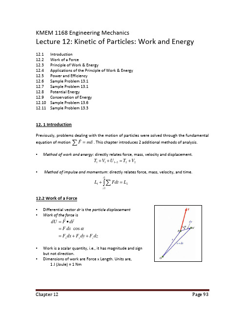
KMEM 1168 Engineering MechanicsLecture 12: Kinetic of Particles: Work and Energy12.1 Introduction 12.2 Work of a Force12.3 Principle of Work & Energy12.4 Applications of the Principle of Work & Energy 12.5 Power and Efficiency 12.6 Sample Problem 13.1 12.7 Sample Problem 13.1 12.8 Potential Energy12.9 Conservation of Energy 12.10 Sample Problem 13.6 12.11 Sample Problem 13.312. 1 IntroductionPreviously, problems dealing with the motion of particles were solved through the fundamentalequation of motion a m F rr =∑. This chapter introduces 2 additional methods of analysis.•Method of work and energy : directly relates force, mass, velocity and displacement. 222111V T U V T +=++−•Method of impulse and momentum : directly relates force, mass, velocity, and time.2121L Fdt L t t =+∫∑12.2 Work of a Force• Differential vector dr is the particle displacement •Work of the force isdzF dy F dx F ds F rd F dU z y x ++==•=αcos r r• Work is a scalar quantity, i.e., it has magnitude and sign but not direction.• Dimensions of work are Force x Length. Units are,1 J (Joule) = 1 Nm• Work of a force during a finite displacement,• Work is represented by the area under the curve of F t plotted against s .• Work of a constant force in rectilinear motion,•Forces which do not do work (ds = 0 or cos a = 0):a) reaction at frictionless pin supporting rotating bodyb) reaction at frictionless surface when body in contact moves along surface c) weight of a body when its center of gravity moves horizontally12.3 Principle of Work & Energy•Consider a particle of mass m acted upon by a force•Integrating from A 1to A 2,•The work of the force is equal to the change in kinetic energy of the particle.• Units of work and kinetic energy are the same:12.4 Applications of the Principle of Work & Energy•The bob is held at point 1 and if we wish to find the velocity of pendulum bob at point 2, we have to consider the method of work and energy. Force P acts normal to path and does no work.•In this method, unlike the method of Newton 2nd Law, we can find velocity without having to determine expression for acceleration and integrating.•All quantities are scalars and can be added directly. Forces which do no work (eg. In this case is the tension in the cord P)are eliminated from the problem. Principle of work and energy cannot be applied to directly determine the acceleration of the pendulum bob.•The tension in the cord is required to supplement the method of work and energy with an application of Newton’s second law.•As the bob passes through A 2,12.5 Power and Efficiency•Power = rate at which work is done.vF dt r d F dt dU r r r r •=•==•Dimensions of power are work/time or force x velocity. Units for power are• Efficiency is the ratio of the power output to the power input,12.6 Sample Problem 13.1An automobile weighing 4000 N is driven down a 5oincline at a speed of 88 m /s when the brakes are applied causing a constant total breaking force of 1500 N.Determine the distance traveled by the automobile as it comes to a stop.• Evaluate the change in kinetic energy.()()m N 15488008810/4000sm 88221212111⋅====mv T v0022==T v•Determine the distance required for the work to equal the kinetic energy change.()()()()x x x U 11515sin 4000150021−=°+−=→()0115115488002211=−=+→x T U Tm 6.1345=x12.7 Sample Problem 13.2Two blocks are joined by an inextensible cable as shown. If the system is released from rest, determine the velocity of block A after it has moved 2 m.Assume that the coefficient of friction between block A and the plane is μk= 0.25 and that the pulley isweightless and frictionless.• Apply the principle of work and energy separately to blocks A and B .Block A:()()()()()()()()()221221221120024902220:N490196225.0N 196281.9200v F vm F F T U T W N F W C A A C A k A k A A =−=−+=+======→µµBlock B:()()()()()()()()2212212211300229402220:N 294081.9300v F vm W F T U T W c B B c B =+−=+−=+==→•When the two relations are combined, the work of the cable forces cancel. Solve for the velocity.()()()()22120024902v F C =−()()()()221300229402v F c =+−()()()()()()2212215004900300200249022940vv=+=− s m 43.4=v12.8 Potential EnergyThere are 2 kinds of potential energyi) Gravitational Potential Energy, V g ii) Elastic Potential Energy, V eGravitational Potential Energy (V g )• Work of the force of gravity W ,2121y W y W U −=→• Work is independent of path followed, it depends only on the initial and final values of W(dy).()()2121g g V V U −=→•Choice of datum from which the elevation y is measured is arbitrary. But always choose the lower position as the datum to avoid negative potential energy. Units of work and potential energy are the same:J m N )(=⋅==dy W V gElastic Potential Energy, V e• Work of the force exerted by a spring dependsonly on the initial and final deflections of the spring,2221212121kx kx U −=→• The potential energy of the body with respect tothe elastic force,()()2121221e e e V V U kxV −==→•Note that the preceding expression for V e is valid only if the deflection of the spring is measured from its undeformed position.=→21U 221kx12.9 Conservation of Energy•Conservation of energy equation,constant2211=+=+=+V T E V T V T• When a particle moves under the action of conservative forces, the total mechanical energy (E) is constant.•Friction forces are not conservative. Total mechanical energy of a system involving friction decreases. Mechanical energy is dissipated by friction into thermal energy or heat.ll W V T W V T =+==11110()ll l W V T V W g g Wmv T =+====22222212022112.10 Sample Problem 13.6A 20-N collar slides without friction along a vertical rod as shown. The spring attached to the collar has an undeflected length of 4 cm and a constant of 3 N/cm. If the collar is released from rest at position 1, determine its velocity after it has moved 6 cm to position 2.• Apply the principle of conservation of energy betweenpositions 1 and 2.Position 1:()()0024cmN 24483112212121=+=+=⋅=−==T V V V kx V g e ePosition 2:()()()()222221222212221102021cm N 6612054cmN 120620cmN 544013v mv T V V V Wy V kx V g e g e ==⋅−=−=+=⋅−=−==⋅=−==•Conservation of Energy:cmN 66cm N 240222211⋅−=⋅++=+v V T V T↓=s m 5.92v12.11 Sample Problem 13.3A spring is used to stop a 60 kg package which is sliding on a horizontal surface. The spring has a constant k = 20 kN/m and is held by cables so that it is initially compressed 120 mm. The package has a velocity of 2.5 m/s in the position shown and the maximum deflection of the spring is 40 mm. Determine(a) the coefficient of kinetic friction between the package and surface(b) the velocity of the package as it passes again through the position shown.(a) Use principle of work and energy equation,NF g N µ==60222111V T U V T +=++→021)(212122212+∆=−∆+x k s N x k mu µ()()222)04.012.0)(20000(2)04.06.0)(60()12.0)(20000(215.26021+=+−+g µ 20.0=µ(b) Apply the principle of work and energy for the rebound of the package.333222V T U V T +=++→ 2323222121)(210x k mv s N x k ∆+=−∆+µ2232)12.0)(20000(21)60(21)64.0)(60)(2.0()16.0)(20000(21+=−v g s m v /11.13=NB: Part B demonstrates that the final velocity at 3 is less than the initial velocity at 1. This is due to the loss of energy due to friction. The total mechanical energy is not conserved.。

Lecture 12: Visualizing and UnderstandingAdministrativeMilestones due tonight on Canvas, 11:59pmMidterm grades released on Gradescope this weekA3 due next Friday, 5/26HyperQuest deadline extended to Sunday 5/21, 11:59pm Poster session is June 6Last Time: Lots of Computer Vision TasksClassification + LocalizationSemantic SegmentationObject DetectionInstance SegmentationCATGRASS , CAT , TREE , SKYDOG , DOG , CATDOG , DOG , CATSingle ObjectMultiple ObjectNo objects, just pixelsThis image is CC0 public domainThis image is CC0 public domainWhat’s going on inside ConvNets?This image is CC0 public domainClass Scores:1000 numbers Input Image:3 x 224 x 224What are the intermediate features looking for?Krizhevsky et al, “ImageNet Classification with Deep Convolutional Neural Networks”, NIPS 2012.Figure reproduced with permission.First Layer: Visualize FiltersAlexNet:64 x 3 x 11 x 11ResNet-18:64 x 3 x 7 x 7ResNet-101:64 x 3 x 7 x 7DenseNet-121:64 x 3 x 7 x 7Krizhevsky, “One weird trick for parallelizing convolutional neural networks”, arXiv 2014 He et al, “Deep Residual Learning for Image Recognition”, CVPR 2016Huang et al, “Densely Connected Convolutional Networks”, CVPR 2017Visualize the filters/kernels (raw weights)We can visualize filters at higher layers, but not that interesting (these are taken from ConvNetJS CIFAR-10 demo)layer 1 weightslayer 2 weightslayer 3 weights16 x 3 x 7 x 720 x 16 x 7 x 720 x 20 x 7 x 7FC7 layerLast Layer4096-dimensional feature vector for an image (layer immediately before the classifier)Run the network on many images, collect the feature vectorsLast Layer: Nearest Neighbors4096-dim vectorTest image L2 Nearest neighbors in feature spaceRecall: Nearest neighborsin pixel spaceKrizhevsky et al, “ImageNet Classification with Deep Convolutional Neural Networks”, NIPS 2012.Figures reproduced with permission.Visualize the “space” of FC7 feature vectors by reducing dimensionality of vectors from 4096 to 2 dimensionsSimple algorithm: Principle Component Analysis (PCA) More complex: t-SNEVan der Maaten and Hinton, “Visualizing Data using t-SNE”, JMLR 2008Figure copyright Laurens van der Maaten and Geoff Hinton, 2008. Reproduced with permission.Van der Maaten and Hinton, “Visualizing Data using t-SNE”, JMLR 2008Krizhevsky et al, “ImageNet Classification with Deep Convolutional Neural Networks”, NIPS 2012. Figure reproduced with permission.See high-resolution versions at/people/karpathy/cnnembed/Visualizing ActivationsYosinski et al, “Understanding Neural Networks Through Deep Visualization”, ICML DL Workshop 2014.Figure copyright Jason Yosinski, 2014. Reproduced with permission.conv5 feature map is128x13x13; visualizeas 128 13x13grayscale imagesMaximally Activating PatchesPick a layer and a channel; e.g. conv5 is128 x 13 x 13, pick channel 17/128Run many images through the network,record values of chosen channelVisualize image patches that correspondto maximal activationsSpringenberg et al, “Striving for Simplicity: The All Convolutional Net”, ICLR Workshop 2015Figure copyright Jost Tobias Springenberg, Alexey Dosovitskiy, Thomas Brox, Martin Riedmiller, 2015;reproduced with permission.Occlusion Experiments Mask part of the image beforefeeding to CNN, draw heatmap ofprobability at each mask locationZeiler and Fergus, “Visualizing and Understanding Convolutional Networks”, ECCV 2014Boat image is CC0 public domain Elephant image is CC0 public domain Go-Karts image is CC0 public domainHow to tell which pixels matter for classification?Dog Simonyan, Vedaldi, and Zisserman, “Deep Inside Convolutional Networks: Visualising Image Classification Modelsand Saliency Maps”, ICLR Workshop 2014.Figures copyright Karen Simonyan, Andrea Vedaldi, and Andrew Zisserman, 2014; reproduced with permission.How to tell which pixels matter for classification?Dog Compute gradient of (unnormalized) classscore with respect to image pixels, takeabsolute value and max over RGB channelsSimonyan, Vedaldi, and Zisserman, “Deep Inside Convolutional Networks: Visualising Image Classification Modelsand Saliency Maps”, ICLR Workshop 2014.Figures copyright Karen Simonyan, Andrea Vedaldi, and Andrew Zisserman, 2014; reproduced with permission.Simonyan, Vedaldi, and Zisserman, “Deep Inside Convolutional Networks: Visualising Image Classification Models and Saliency Maps”, ICLR Workshop 2014.Figures copyright Karen Simonyan, Andrea Vedaldi, and Andrew Zisserman, 2014; reproduced with permission.Saliency Maps: Segmentation without supervision Simonyan, Vedaldi, and Zisserman, “Deep Inside Convolutional Networks: Visualising Image Classification Modelsand Saliency Maps”, ICLR Workshop 2014.Figures copyright Karen Simonyan, Andrea Vedaldi, and Andrew Zisserman, 2014; reproduced with permission.Rother et al, “Grabcut: Interactive foreground extraction using iterated graph cuts”, ACM TOG 2004Use GrabCut onsaliency mapPick a single intermediate neuron, e.g. onevalue in 128 x 13 x 13 conv5 feature mapCompute gradient of neuron value with respectto image pixelsZeiler and Fergus, “Visualizing and Understanding Convolutional Networks”, ECCV 2014Springenberg et al, “Striving for Simplicity: The All Convolutional Net”, ICLR Workshop 2015Pick a single intermediate neuron, e.g. onevalue in 128 x 13 x 13 conv5 feature mapCompute gradient of neuron value with respectto image pixelsImages come out nicer if you onlybackprop positive gradients througheach ReLU (guided backprop)ReLUZeiler and Fergus, “Visualizing and Understanding Convolutional Networks”, ECCV 2014 Springenberg et al, “Striving for Simplicity: The All Convolutional Net”, ICLR Workshop 2015Figure copyright Jost Tobias Springenberg, Alexey Dosovitskiy, Thomas Brox, Martin Riedmiller, 2015; reproduced with permission.Zeiler and Fergus, “Visualizing and Understanding Convolutional Networks”, ECCV 2014Springenberg et al, “Striving for Simplicity: The All Convolutional Net”, ICLR Workshop 2015Figure copyright Jost Tobias Springenberg, Alexey Dosovitskiy, Thomas Brox, Martin Riedmiller, 2015; reproduced with permission.(Guided) backprop: Find the part of an image that a neuron responds to Gradient ascent: Generate a synthetic image that maximally activates a neuronI* = arg maxIf(I) + R(I)Neuron value Natural image regularizer1.Initialize image to zerosscore for class c (before Softmax) zero imageRepeat:2. Forward image to compute current scores3. Backprop to get gradient of neuron value with respect to image pixels4. Make a small update to the imageSimple regularizer: Penalize L2norm of generated imageSimonyan, Vedaldi, and Zisserman, “Deep Inside Convolutional Networks: Visualising Image Classification Models and Saliency Maps”, ICLR Workshop 2014.Figures copyright Karen Simonyan, Andrea Vedaldi, and Andrew Zisserman, 2014; reproduced with permission.Simple regularizer: Penalize L2norm of generated imageSimonyan, Vedaldi, and Zisserman, “Deep Inside Convolutional Networks: Visualising Image Classification Models and Saliency Maps”, ICLR Workshop 2014.Figures copyright Karen Simonyan, Andrea Vedaldi, and Andrew Zisserman, 2014; reproduced with permission.Simple regularizer: Penalize L2norm of generated imageYosinski et al, “Understanding Neural Networks Through Deep Visualization”, ICML DL Workshop 2014. Figure copyright Jason Yosinski, Jeff Clune, Anh Nguyen, Thomas Fuchs, and Hod Lipson, 2014. Reproduced with permission.Better regularizer: Penalize L2 norm of image; also during optimization periodically(1)Gaussian blur image(2)Clip pixels with small values to 0(3)Clip pixels with small gradients to 0 Yosinski et al, “Understanding Neural Networks Through Deep Visualization”, ICML DL Workshop 2014.Better regularizer: Penalize L2 norm ofimage; also during optimizationperiodically(1)Gaussian blur image(2)Clip pixels with small values to 0(3)Clip pixels with small gradients to 0Yosinski et al, “Understanding Neural Networks Through Deep Visualization”, ICML DL Workshop 2014.Figure copyright Jason Yosinski, Jeff Clune, Anh Nguyen, Thomas Fuchs, and Hod Lipson, 2014. Reproduced with permission.Better regularizer: Penalize L2 norm ofimage; also during optimizationperiodically(1)Gaussian blur image(2)Clip pixels with small values to 0(3)Clip pixels with small gradients to 0Yosinski et al, “Understanding Neural Networks Through Deep Visualization”, ICML DL Workshop 2014.Figure copyright Jason Yosinski, Jeff Clune, Anh Nguyen, Thomas Fuchs, and Hod Lipson, 2014. Reproduced with permission.Use the same approach to visualize intermediate featuresYosinski et al, “Understanding Neural Networks Through Deep Visualization”, ICML DL Workshop 2014.Figure copyright Jason Yosinski, Jeff Clune, Anh Nguyen, Thomas Fuchs, and Hod Lipson, 2014. Reproduced with permission.Use the same approach to visualize intermediate featuresYosinski et al, “Understanding Neural Networks Through Deep Visualization”, ICML DL Workshop 2014.Figure copyright Jason Yosinski, Jeff Clune, Anh Nguyen, Thomas Fuchs, and Hod Lipson, 2014. Reproduced with permission.Adding “multi-faceted” visualization gives even nicer results:(Plus more careful regularization, center-bias)Nguyen et al, “Multifaceted Feature Visualization: Uncovering the Different Types of Features Learned By Each Neuron in Deep Neural Networks”, ICML Visualization for Deep Learning Workshop 2016. Figures copyright Anh Nguyen, Jason Yosinski, and Jeff Clune, 2016; reproduced with permission.Figures copyright Anh Nguyen, Jason Yosinski, and Jeff Clune, 2016; reproduced with permission.Optimize in FC6 latent space instead of pixel space:Nguyen et al, “Synthesizing the preferred inputs for neurons in neural networks via deep generator networks,” NIPS 2016Figure copyright Nguyen et al, 2016; reproduced with permission.(1)Start from an arbitrary image(2)Pick an arbitrary class(3)Modify the image to maximize the class(4)Repeat until network is fooledBoat image is CC0 public domain Elephant image is CC0 public domainWhat is going on? Ian Goodfellow will explain Boat image is CC0 public domainElephant image is CC0 public domainRather than synthesizing an image to maximize a specific neuron, insteadtry to amplify the neuron activations at some layer in the networkChoose an image and a layer in a CNN; repeat:1.Forward: compute activations at chosen layer2.Set gradient of chosen layer equal to its activation3.Backward: Compute gradient on image4.Update imageMordvintsev, Olah, and Tyka, “Inceptionism: Going Deeper into NeuralNetworks”, Google Research Blog. Images are licensed under CC-BY4.0Rather than synthesizing an image to maximize a specific neuron, instead try to amplify the neuron activations at some layer in the networkEquivalent to:I* = arg max I ∑i f i (I)2Mordvintsev, Olah, and Tyka, “Inceptionism: Going Deeper into Neural Networks”, Google Research Blog . Images are licensed under CC-BY 4.0Choose an image and a layer in a CNN; repeat:1.Forward: compute activations at chosen layer 2.Set gradient of chosen layer equal to its activation 3.Backward: Compute gradient on image 4.Update imageCode is very simple but it uses a couple tricks: (Code is licensed under Apache 2.0)Code is very simple but it uses a couple tricks: (Code is licensed under Apache 2.0)Jitter imageCode is very simple but it uses a couple tricks: (Code is licensed under Apache 2.0)Jitter imageL1 Normalize gradientsCode is very simple butit uses a couple tricks:(Code is licensed under Apache 2.0)Jitter imageL1 Normalize gradientsClip pixel valuesAlso uses multiscale processing for a fractal effect (not shown)Sky image is licensed under CC-BY SA 3.0Image is licensed under CC-BY 4.0Image is licensed under CC-BY 4.0Image is licensed under CC-BY 3.0Image is licensed under CC-BY 3.0Image is licensed under CC-BY 4.0Given a CNN feature vector for an image, find a new image that: -Matches the given feature vector-“looks natural” (image prior regularization)Mahendran and Vedaldi, “Understanding Deep Image Representations by Inverting Them”, CVPR 2015Given feature vectorFeatures of new imageTotal Variation regularizer (encourages spatial smoothness)Reconstructing from different layers of VGG-16Mahendran and Vedaldi, “Understanding Deep Image Representations by Inverting Them”, CVPR 2015Figure from Johnson, Alahi, and Fei-Fei, “Perceptual Losses for Real-Time Style Transfer and Super-Resolution”, ECCV 2016. Copyright Springer, 2016.Reproduced for educational purposes.。