第7章 补充01—传递矩阵法
- 格式:ppt
- 大小:1.49 MB
- 文档页数:12


Transfer Matrix MethodG.Eric Moorhouse,University of WyomingReference:Transfer Matrix MethodI.M.Gessel and R.P.Stanley,‘Algebraic Enu-meration’,in Handbook of Combinatorics Vol.2, ed.R.L.Graham et al.,Elsevier,1995,pp.1021–1061.References:Dimensions of CodesN.Hamada,‘The rank of the incidence matrixof points and d-flats infinite geometries’,J. Sci.Hiroshima Univ.Ser.A-I32(1968),381–396.M.Bardoe and P.Sin,‘The permutation mod-ules for GL(n+1,q)acting on P n(q)and F n+1q’,to appear in JLMS./~sin/preprints/hamada.dviG.E.Moorhouse,‘Dimensions of Codes from Finite Projective Spaces’(as html and as Maple worksheet)/~moorhous/src/hamada.html /~moorhous/src/hamada.mwsProblem1Let S k be the set of‘words’of length k consist-ing of‘a’s and‘b’s,with no two consecutive ‘b’s.Determine F k=|S k|.F0=1‘’F1=2‘a’‘b’F2=3‘aa’‘ab’‘ba’F3=5‘aaa’‘aab’‘aba’‘baa’‘bab’F4=8‘aaaa’‘aaab’‘aaba’‘abaa’‘abab’‘baaa’‘baab’‘baba’etc.This gives all but thefirst term of the Fibonacci sequence1,1,2,3,5,8,13,21,34,55,89,144,...To find a formula for F k ,we work instead with the generating function∞k =0F k t k =1+2t +3t 2+5t 3+8t 4+13t 5+···Observe that words w ∈S k correspond to paths of length k ,starting at vertex 1in the digraph12..................................................................................................................................................................................................................................................................................................................................................................................................................................................................................................................................................................................................................................................................................................................................................................................................................................................................................................................................................................append ‘a’append ‘a’append ‘b’Words not ending in ‘b’Words ending in ‘b’Agenda1.Motivating Problem1(above)2.Counting Walks by the Transfer Matrix Method3.Application to Problem14.Counting Closed Walks5.Counting Weighted Walks in Digraphs withWeighted Edges6.MAPLE Worksheet for Problem17.Application to Coding TheoryThe Transfer Matrix Method Let D be a digraph (directed graph),possibly with loops,having vertices 1,2,3,...,n .Let A =[a ij :1≤i,j ≤n ]be the adjacency matrix of D ;in other words,a ij = 1,if (i,j )is an edge of D ;0,otherwise.A walk of length k in D is a sequence......................................................................................................................................................................................................................................................................................................................................···◦◦◦◦i 0i 1i 2i k→→→→of (not necessarily distinct)vertices such that each ...........................................................................................◦◦i r −1i r →is an edge of D .Counting Walks from i to jLet w ij(k)be the number of walks of length k from vertex i to vertex j in D.Then w ij(k)is the(i,j)-entry of A k.This is readily computed by reading offthe coefficient of t k in the gen-erating function k≥0w ij(k)t k which in turn is the(i,j)-entry of(I−tA)−1=I+tA+t2A2+t3A3+···. Since the(i,j)-entry of(I−tA)−1is of the formpoly.in t of degree≤n−1det(I−tA),w ij(k)satisfies a linear recurrencew ij(k+n)=n−1r=0c r w ij(k+r)for all k≥0where det(I−tA)=1−c n−1t−c n−2t2−···−c0t n.The initial conditions w ij(0),w ij(1),..., w ij(n−1)depend on i and j but the recurrence does not.Counting All WalksLet w(k)= n i=1 n j=1w ij(k),the total num-ber of walks of length k.This is the coefficient of t k in the sum of the entries of(I−tA)−1.In particular w(k)satisfies the same recurrence as the w ij(k)’s:w(k+n)=n−1r=0c r w(k+r)for all k≥0but with different initial conditions.Counting Closed WalksLet w closed(k)= n i=1w ii(k),the total number of closed walks of length k(i.e.starting and ending at the same vertex).This is the coef-ficient of t k in trace((I−tA)−1).In particular w closed(k)satisfies the same linear recurrence as the w ij(k)’s and w(k),but again with different initial conditions.Here we assumed the initial/final vertex to be distinguished,i.e.the walks(i0,i1,i2,...,i k)and (i1,i2,...,i k,i0)are counted as distinct unless all i0=i1=···=i k.ExampleLet F k be the number of‘words’of length k consisting of‘a’s and‘b’s,with no two con-secutive‘b’s.F0=1‘’F1=2‘a’‘b’F2=3‘aa’‘ab’‘ba’F3=5‘aaa’‘aab’‘aba’‘baa’‘bab’F4=8‘aaaa’‘aaab’‘aaba’‘abaa’‘abab’‘baaa’‘baab’‘baba’etc.This gives all but thefirst term of the Fibonacci sequence1,1,2,3,5,8,13,21,34,55,89,144,...Observe that F k is the number of paths of length k ,starting at vertex 1in the digraph12.................................................................................................................................................................................................................................................................................................................................................................................................................................................................................................................................................................................................................................................................................................................................................................................................................................................................................................................................................................append ‘a’append ‘a’append ‘b’Words not ending in ‘b’Words ending in ‘b’A = 111(I −tA )−1=11−t −t 2 1t t 1−tk ≥0F k t k =sum of (1,1)-and (1,2)-entries of (I −tA )−1=1+t 1−t −t 2=1√5 α21−αt −β21−βt=1√5 k ≥0(αk +2−βk +2)t k where α=(1+√5)/2,β=(1−√5)/2.From (1−t −t 2) k ≥0F k t k =1+t we obtainF k = 1,if k =0;2,if k =1;F k −1+F k −2,if k ≥2so by induction,F k is the (k +1)st Fibonacci number.From the series expansion we obtain the explicit formulaF k =αk +2−βk +2√5for k ≥0.Wraparound VersionLet L k(for k≥0)be the number of‘words’of length k consisting of‘a’s and‘b’s with no consecutive‘b’s,and which do not both start and end with‘b’.For technical reasons we will take L0=2.For k≥2,we are simply counting necklaces with a mber and b lack beads having no two consecutive black beads;however,each neck-lace has a distinguished starting point(a knot in its cord)and a distinguished direction(clock-wise or counter-clockwise).L1=1‘a’L2=3‘aa’‘ab’‘ba’L3=4‘aaa’‘aab’‘aba’‘baa’L4=7‘aaaa’‘aaab’‘aaba’‘abaa’‘abab’‘baaa’‘baba’These are the familiar Lucas numbers which satisfy the same recurrence relation as the Fi-bonacci numbers,but a different initial condi-tion.Note that L k is the number of closed walks of length k in our digraph.k ≥0L k t k =trace ((I −tA )−1)=2−t 1−t −t 2=11−αt +11−βt=k ≥0(αk +βk )t kFrom (1−t −t 2) k ≥0L k t k =2−t we obtainL k = 2,if k =0;1,if k =1;L k −1+L k −2,if k ≥2From the series expansion we obtain the ex-plicit formulaL k=αk+βk for k≥0.Counting Walks with Weighted Edges As before,D is a digraph (directed graph),pos-sibly with loops,having vertices 1,2,3,...,n .Assign a weight to each edge:...........................................................................................◦◦i j →a ij (Non-edges have weight zero.)Define the weight of a walk......................................................................................................................................................................................................................................................................................................................................···◦◦◦◦i 0i 1i 2i k →→→→a i 0i 1a i 1i 2a i 2i 3a i k −1i k of length k to be the producta i 0i 1a i 1i 2a i 2i 3···a i k −1i k .Let A =[a ij :1≤i,j ≤n ].Thenw ij(k):=The sum of all weightsof walks in D of length k from vertex i to vertex j=(i,j)-entry of A khas generating function k≥0w ij(k)t k equal to the(i,j)-entry of(I−tA)−1=I+tA+t2A2+t3A3+···as before.ExampleWe have determined the number F k of words of length k consisting of‘a’s and‘b’s,with no two consecutive‘b’s.How many such words contain r‘a’s and(therefore)k−r‘b’s?12.................................................................................................................................................................................................................................................................................................................................................................................................................................................................................................................................................................................................................................................................................................................................................................................a ab A = a b a0 (I −tA )−1=11−at −abt 2 1bt at 1−atThe sum of the (1,1)-and (1,2)-entries is1+bt1−at −abt 2=1+(a +b )t +(a 2+2ab )t 2+(a 3+3a 2b +ab 2)t 3+(a 4+4a 3b +3a 2b 2)t 4+···Thus,for example,among the F 4=8words of length 4,1has 4‘a’s and 0‘b’s;4have 3‘a’s and 1‘b’;3have 2‘a’s and 2‘b’s.Codes from Finite GeometryConsider the projective plane of order 2:•••••••a bc d e f g ..........................................................................................................................................................................................................................................................................................................................................................................................................................................................................................................................................................................................................................................................................................................................................................................................................................................................................................................................................................................................................................................................................................................................................................................................................................................................................The binary code of this geometry is the sub-space C ≤F 7(where F ={0,1}mod 2)spanned by the lines:a b c d e f g a b c d e f g C ={0000000,1111111,1101000,0010111,0110100,1001011,0011010,1100101,0001101,1110010,1000110,0111001,0100011,1011100,1010001,0101110}|C|=24;dim C =4The code above is the 1-error correcting binary Hamming code of length 7.The projective plane is constructed from F 3by taking as points and lines the 1-and 2-dimensional subspaces of F 3.•••••••001010100011110111101.........................................................................................................................................................................................................................................................................................................................................................................................................................................................................................................................................................................................................................................................................................................................................................................................................................................................................................................................................................................................................................................................................................................................................................................................................................................................................Codes of Finite Projective SpacesLet F be thefield of order p e,p prime.Pro-jective n-space over F has as its points,lines, etc.the subspaces of F n+1of dimension1,2, etc.Problem:Compute the dimension of the code C=C n,p,e,k spanned by the subspaces of codi-mension k.Solution by Hamada’s Formula(the follow-ing theorem)is usually computationally infea-sible.Solution by the Transfer Matrix MethodTheorem(Bardoe and Sin,1999)Define M(t)=(1+t+t2+···+t p−1)n+1.Let D=D n,p,e,k be the digraph with vertices 1,2,...,k,and the edge from vertex i to vertex j has weight equal to the coefficient of t pj−i in M(t).Thendim C n,p,e,k=1+sum of weights of closed walks of length ein D=1+ coeff.of t ein tr[(I−tA)−1]where A is the k×k matrix whose(i,j)-entry is the weight of edge(i,j)(defined above).Example:Projective Plane of Order2C=binary code spanned by the seven lines (subspaces of codimension k=1)M(t)=(1+t)3=1+3t+3t2+t3A=[3](coefficient of t1in M(t))(I−tA)−1= 1 1−3ttr[(I−tA)−1]=11−3t=1+3t+9t2+27t3+···dim C=1+3=4。

传递矩阵法是研究转子系统动力学问题的有效手段。
传递矩阵法还具有其它方法(如摄动有限元素法)无法比拟的优点,例如,在做转子系统的临界转速、阻尼固有频率和稳定性计算分析时,由于流体密封交叉刚度、油膜轴承、阻尼项往往是不对称的,再加上陀螺力矩的影响;这样,用随机有限元素法形成的单元刚度矩阵和系统总体刚度矩矩阵往往也是不对称的,阻尼也不可以简单地以小阻尼或比例阻尼系统来替代,求解这样一个非对称系统的复特征值问题,目前还没有一个较为理想的方法。
而传递矩阵法没有随机有限元法在求解这些的问题时带来的这些困难。
因此,传递矩阵法在转子系统动力学问题的研究中占有主导的地位。

传递矩阵法matlab程序传递矩阵法是一种用于计算机程序中传递和操作矩阵的方法,在Matlab中,它被广泛应用于矩阵运算和数据处理等领域。
本文将介绍传递矩阵法的原理和在Matlab中的具体实现。
传递矩阵法是一种通过矩阵传递来操作数据的方法。
它的基本原理是将需要进行操作的数据存储在矩阵中,然后通过矩阵的传递,实现对数据的处理和计算。
这种方法的优势在于可以利用矩阵的高效运算能力,简化程序的编写和调试过程。
在Matlab中,可以使用矩阵操作函数来实现传递矩阵法。
例如,可以使用矩阵的乘法运算来实现矩阵的传递。
假设我们有两个矩阵A 和B,我们希望将矩阵A的数据传递给矩阵B,可以使用如下的Matlab代码实现:```B = A;```这样,矩阵B就完全复制了矩阵A的数据。
通过这种方式,我们可以在程序中传递矩阵,进行各种操作和计算。
除了简单的传递,传递矩阵法还可以实现更复杂的操作。
例如,可以通过传递矩阵进行矩阵的相加、相减、相乘等运算。
假设我们有两个矩阵A和B,我们希望将它们相加得到矩阵C,可以使用如下的Matlab代码实现:```C = A + B;```这样,矩阵C的每个元素都等于矩阵A和矩阵B对应元素的和。
通过传递矩阵法,我们可以很方便地实现这样的矩阵运算。
除了矩阵的运算,传递矩阵法还可以用于数据处理和分析。
例如,可以通过传递矩阵来实现数据的转置、截取、排序等操作。
假设我们有一个矩阵A,我们希望将它的每一列按照从大到小的顺序进行排序,可以使用如下的Matlab代码实现:```B = sort(A,'descend');```这样,矩阵B的每一列都按照从大到小的顺序进行了排序。
通过传递矩阵法,我们可以在Matlab中进行各种复杂的数据处理和分析。
传递矩阵法在Matlab中的应用非常广泛。
无论是矩阵运算、数据处理还是图像处理,都可以通过传递矩阵法来实现。
它不仅提高了程序的效率和可读性,还简化了程序的编写和调试过程。
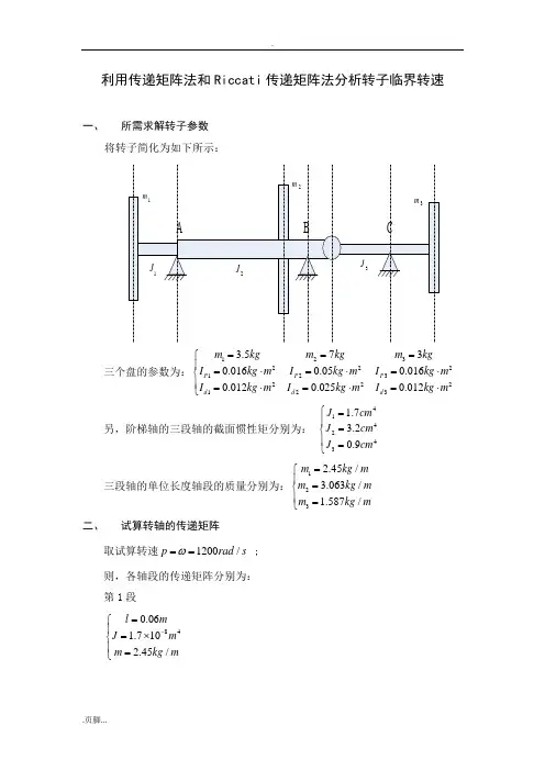
利用传递矩阵法和Riccati 传递矩阵法分析转子临界转速一、所需求解转子参数将转子简化为如下所示:三个盘的参数为:1232221232221230.0160.050.0160.0120.0250.012P P P d d d I kg m I kg m I kg m I kg m I kg m I kg m ⎪=⋅=⋅=⋅⎨⎪=⋅=⋅=⋅⎩ 另,阶梯轴的三段轴的截面惯性矩分别为: 414243 1.73.20.9J cm J cm J cm ⎧=⎪=⎨⎪=⎩三段轴的单位长度轴段的质量分别为:1232.45/3.063/1.587/m kg m m kg m m kg m =⎧⎪=⎨⎪=⎩二、 试算转轴的传递矩阵取试算转速1200/p rad s ω== ; 则,各轴段的传递矩阵分别为: 第1段840.061.7102.45/l m J m m kg m -=⎧⎪=⨯⎨⎪=⎩1 1.0006e+000 6.0007e-002 5.2943e-007 1.0588e-008 3.7356e-002 1.0006e+000 1.7649e-005 5.2943e-007 6.3506e+003 1.2701e+002 1.0006e+000 6.0007e-002 2.1170e+005 6.3506e+003 3.7356e-002 H = 1.0006e+000⎧⎪⎪⎨⎪⎪⎩ 第2段840.153.2103.063/l m J m m kg m -=⎧⎪=⨯⎨⎪=⎩2 1.0145e+000 1.5044e-001 1.7595e-006 8.7927e-008 3.8782e-001 1.0145e+000 2.3506e-005 1.7595e-006 4.9669e+004 2.4821e+003 1.0145e+000 1.5044e-001 6.6353e+005 4.9669e+004 3.8782e-001 H = 1.0145e+000⎧⎪⎪⎨⎪⎪⎩ 第3段840.053.2103.063/l m J m m kg m -=⎧⎪=⨯⎨⎪=⎩3 1.0002e+000 5.0002e-002 1.9531e-007 3.2552e-009 1.4358e-002 1.0002e+000 7.8128e-006 1.9531e-007 5.5135e+003 9.1890e+001 1.0002e+000 5.0002e-002 2.2054e+005 5.5135e+003 1.4358e-002 H = 1.0002e+000⎧⎪⎪⎨⎪⎪⎩ 第4段840.033.2103.063/l m J m m kg m -=⎧⎪=⨯⎨⎪=⎩4 1.0000e+000 3.0000e-002 7.0313e-008 7.0313e-010 3.1013e-003 1.0000e+000 4.6875e-006 7.0313e-008 1.9848e+003 1.9848e+001 1.0000e+000 3.0000e-002 1.3232e+005 1.9848e+003 3.1013e-003 H = 1.0000e+000⎧⎪⎪⎨⎪⎪⎩ 第5段840.10.9101.587/l m J m m kg m -=⎧⎪=⨯⎨⎪=⎩5 1.0053e+000 1.0011e-001 2.7788e-006 9.2607e-008 2.1163e-001 1.0053e+000 5.5614e-005 2.7788e-006 1.1430e+004 3.8094e+002 1.0053e+000 1.0011e-001 2.2877e+005 1.1430e+004 2.1163e-001 H = 1.0053e+000⎧⎪⎪⎨⎪⎪⎩ 第6段840.060.9101.587/l m J m m kg m -=⎧⎪=⨯⎨⎪=⎩6 1.0007e+000 6.0008e-002 1.0000e-006 2.0000e-008 4.5706e-002 1.0007e+000 3.3338e-005 1.0000e-006 4.1137e+003 8.2272e+001 1.0007e+000 6.0008e-002 1.3714e+005 4.1137e+003 4.5706e-002 H = 1.0007e+000⎧⎪⎪⎨⎪⎪⎩ 此6段传递矩阵均采用MATLAB 编程求解,MATLAB 的源文件为H.m 三、采用传递矩阵法进行各段轴的状态参数的传递初始参数列阵为:0101010120101012011Pd d X X I I p M p I Q mp x θθωθ⎛⎫⎛⎫ ⎪⎪ ⎪ ⎪ ⎪=⎛⎫ ⎪-- ⎪⎪ ⎪ ⎪⎝⎭⎝⎭ ⎪⎝⎭令011X =,则初始矩阵可化为:010*******.046e θθ⎛⎫⎪⎪ ⎪ ⎪⎝⎭以初始矩阵乘第一轴段的传递矩阵,则可得第一段轴的终端状态参数:1011011011010.06306+ 1.0541.102 +5890 3.0885 26566.0 5..7062556k k k k e e X M Q θθθθθ⎛⎫⎛⎫⎪ ⎪ ⎪ ⎪= ⎪ ⎪ ⎪ ++⎪⎝⎭⎝⎭由于考虑支座的支撑刚度系数变化从5101*101*10,先取51*10,那么100001000010001KK k⎡⎤⎢⎥⎢⎥=⎢⎥⎢⎥-⎣⎦,此处510k =,则可得支座A 后第2段的起始端参数阵为: 020102010201560201 0.06306 + 1.0541.102 + 5890.0 3.088*10260.2 5.149*2.01076X M Q θθθθθ⎛⎫⎛⎫ ⎪ ⎪ ⎪ ⎪= ⎪ ⎪⎪ ++⎪⎝⎭⎝⎭用第2段的传递矩阵乘此矩阵,可得第2段终端参数:20120120120166 0.2402+ 2.4721.282 + 19.11900.0 1.147*1099133.0 6.170477*1k k k k X M Q θθθθθ⎛⎫⎛⎫ ⎪ ⎪ ⎪ ⎪= ⎪ ⎪ ⎪ ⎪⎝⎭⎝⎭++用中间圆盘的传递矩阵乘第2段终端参数阵,即可得第3段起始端参数:03010306103016307010.2402 + 2.472 1.282 + 1958022.0 1.848*102.52*10 3.11*10.47X M Q θθθθθ+⎛⎫⎛⎫ ⎪ ⎪ ⎪ ⎪= ⎪ ⎪⎪ ⎭⎝⎭+⎪⎝ 用第3段传递矩阵乘其始端参数矩阵:'013'013'013'6356017 0.3238 + 3.9092.231+ 401.855*10 3.419*102.581*10 3.178*10.02k k k k X M Q θθθθθ⎛⎫⎛⎫ ⎪ ⎪⎪ ⎪= ⎪ ⎪⎪ ⎪⎪⎝⎭++⎝⎭ 用上式乘以支座刚度矩阵,得其终端参数:01305667130130130.3238 + 3.9092.231 + 40.01.855*10 3.419*102.549*10 3.1392*10k k k k X M Q θθθθθ⎛⎫⎛⎫⎪ ⎪⎪ ⎪= ⎪ ⎪⎪ ⎪ ⎝⎭⎭+⎪+⎝ 则,根据可得: ,则可得支座B 后第4段的起始端参数阵为:560104010401040104670.3238 + 3.9092.231 + 40.01.855*10 3.419*102.549*10 3.139*102X M Q θθθθθ⎛⎫⎛⎫ ⎪ ⎪⎪ ⎪= ⎪ ⎪⎪ ⎪⎪⎝⎭⎝++⎭ 同上,用此段轴的传递函数乘其起始端的状态参数,可得:4014014014015667 0.4056 + 5.372 3.281 + 582.626*10 4.369*102.597*10 3..172*20k k k k X M Q θθθθθ+⎛⎫⎛⎫⎪ ⎪ ⎪ ⎪= ⎪ ⎪⎪ ⎪⎝⎭⎝⎭+则,根据40k M =可得:01-16.64θ= 则,可得第5段的起始参数矩阵:050750505-1.3753.69601.12*10X M Q θ⎛⎫⎛⎫ ⎪ ⎪ ⎪ ⎪= ⎪ ⎪ ⎪ ⎭⎝-⎪⎝⎭ 其中,5θ为铰链处的转角。

多体系统传递矩阵法及其应用多体系统是由许多互相作用的体组成的复杂体系,如分子、原子、晶体等。
传递矩阵法是一种处理多体系统的方法,它能够高效地计算多体系统在空间中的相互作用关系,是现代物理学研究中不可或缺的重要手段。
传递矩阵法最早应用于固体物理领域中的声子传输问题。
其基本思想是通过计算相邻体间的相互作用关系,得出整个体系中体与体之间的传递矩阵。
具体来说,传递矩阵法假设每个体以弹性球体为模型,并将每个弹性球体中储存的平面波能量互相传递,形成整个体系中的传递矩阵。
这种方法在研究固体中光声声子的传输、声子光子的散射等问题中具有重要的应用价值。
除了固体物理领域,传递矩阵法还广泛应用于原子、分子的电子结构计算以及化学反应机理的模拟等领域。
计算和分析分子/团簇数据在化学特异性中的作用是大量分子和聚集体计算化学和物理学领域的重要问题。
基于传递矩阵法可以对分子结构、物理特性以及从催化到切削的各种机械和电子反应进行分析和预测。
在实际应用中,传递矩阵法的计算和建模过程也面临着许多挑战,如有限的计算能力、模型精度等问题。
为了解决这些问题,一些改进的传递矩阵法,如多重散射和Greens函数方法等也被提出,以提高计算精度和效率。
同时,也有越来越多的科研工作者尝试将传递矩
阵法与机器学习等前沿技术相结合,从而拓展传递矩阵法的应用范围和精度,实现更加智能化的计算和数据分析。
总之,传递矩阵法在物理、化学、材料学、和计算机科学等领域都扮演着重要的角色。
通过该方法,我们可以更加深入地理解多体系统内部的相互作用关系,进而更好地预测和优化系统的性质和行为,为理论和实践应用提供了新的思路和创新性解决方案。
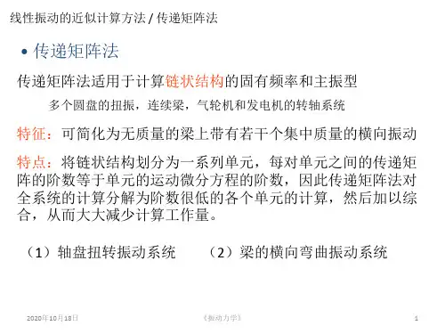
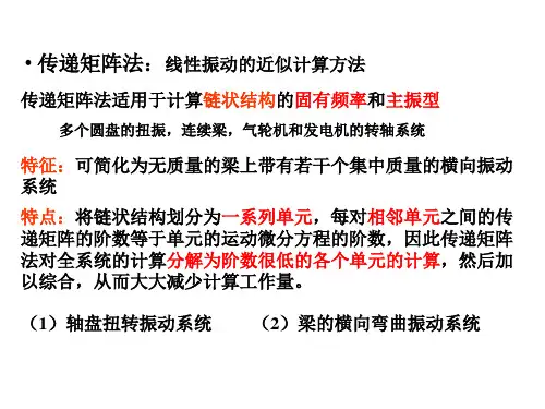
传递矩阵法
传递矩阵法,也称为状态转移矩阵法,是一种用来求解动态规划问题的方法。
它是将原问题分成多段子问题,每一段子问题都可以用状态转移矩阵表示,最后把多个子问题求解出来,并最终组合在一起,得到最优解的方法。
传递矩阵法是动态规划中最常使用的一种方法,它的核心思想是:将原问题分解成小问题,然后将小问题求解出来,最后再组合在一起,求出最优解。
传递矩阵法的具体步骤如下:
1、分析问题:对需要求解的问题进行分析,找出问题的目标函数,状态转移方程式,以及约束条件。
2、构建状态转移矩阵:根据上述分析结果,构建状态转移矩阵,并填充状态转移方程式中的变量,形成状态转移矩阵。
3、求解状态转移矩阵:对状态转移矩阵进行求解,根据问题的特点,可以采用递推法、回溯法、逐步增加法等求解方法,求解出状态转移矩阵。
4、解决问题:根据求解出来的状态转移矩阵,解决问题,得到最优解。
传递矩阵法是一种求解动态规划问题的非常常用的方法,其优点是可以将原问题分解成小问题,并将小问题求
解出来,最后再组合在一起,求出最优解,比较简单易行。
但是其缺点也很明显,需要分析的问题必须能够被分解成小问题。
此外,传递矩阵法的时间复杂度依然较大,所以在解决复杂问题时,可能会遇到时间上的限制。
4.传递矩阵法4.1传递矩阵法对泵轴的弯曲振动分析如图所示,将主轴简化个简支梁模型,一端固定,另一端自由n 级阶梯圆柱。
在最右端作用有弯矩n M ,轴向力n N 。
各阶柱长度为i L ,惯性矩为i I ,弹性模量为E ,这些量为已知量。
1)现用传递矩阵法研究阶梯柱。
将阶梯轴分成若干单元。
按照截面的不同,将阶梯轴分成12,,.......n x x x 个单元。
使每一节轴的截面相等。
2)去其中1x 单元进行受力分析,得出该单元的传递矩阵。
1.单元的受力情况,坐标系统和质量值如图所示。
把该单元每个横截面上的挠度y 、转角0=y '、弯矩M 、铀向力N 构成一状态矢量{()}[(),(),(),()]T U x y x y x M x N x '=。
如在该单元的x=0的截面上状态矢量为00000{},,,TU y y M N ⎡⎤'=⎣⎦,在x=1L 的截面上状态矢量为1]111{},,,T U y y M N '⎡⎤=⎣⎦。
该单元任一截面x 的弯矩0()()o o M x M N y y =--其绕曲线微分方程为10()()o o EI y x M N y y ''=+-4-1-1将(4-1-1)整理简化,(其中211oN k EI =)。
2201101()M y k y k y N ''+=+4-1-2 利用在结构力学中的常系数微分方程的初参数解,求出4-1-2式的通解为下式00111sin (1cos )o oy My y k x k x k N '=++- 4-1-3对4-1-3求导得:111cos sin ooM y y k x k k x N ''=+ 4-1-4对4-1-4求导:21110sin cos o l M y y k k x k k x N '''=-+ 4-1-5 故101111()sin cos N o M x EI y y EI k k x M k x '==-+ 4-1-6 由x 轴方向的平衡条件可得:01()N N N x ==4-1-7由4-1-3,4-1-4,4-1-6,4-1-7得矩阵形式11111001111011110sin 1cos 10()()sin 0cos 0()0sin cos 0()0000k x k x k EI k y y x y y x k x k x EI k M M x EI k k xk x N N x -⎡⎤⎢⎥⎧⎫⎧⎫⎢⎥⎪⎪⎪⎪''⎢⎥⎪⎪⎪⎪=⎨⎬⎨⎬⎢⎥⎪⎪⎪⎪⎢⎥⎪⎪⎪⎪⎢⎥-⎩⎭⎩⎭⎢⎥⎣⎦4-1-8或写成 10{()}[()]{}U x W x U = 4-1-9(9)式中{ U}o,{ U(x)}分别为该单元始端截面及任一截面的状态矢量。
典型的传递矩阵计算方法有Myklestad-Prohl传递矩阵法和Riccati传递矩阵法。
Myklestad-Prohl传递矩阵法有很多优点,如矩阵的维数不会随着转子系统的自由度数的增加而增加、计算效率高、程序设计简单、占用内存少等等,所以在实际工程中得到了很广泛的应用。
但是,这种方法在大量应用的过程中,人们发现这种方法也存在一些问题,就是当计算的频率较高、或者结构支承的刚度很大、或者结构的自由度较多时,会出现数值不稳定的现象,从而使计算分析结果的精度大大下降[2~3,39~40]。
为此,1978年Horner和Pilley提出了Riccati传递矩阵法[39],这种方法保留了Myklestad-Prohl传递矩阵法的全部优点,且计算精度高,数值上也比较稳定。
Riccati传递矩阵法在使用过程中遇到的另一个问题是在特征根的搜索过程中剩余量有许多无穷大奇点,因此可能产生增根现象,1987年王正在研究了这一现象后给出了这种奇点的消除方法[40]。
传输矩阵法一、 传输矩阵法概述 1. 传输矩阵在介绍传输矩阵的模型之前,首先引入一个简单的电路模型。
如图1(a)所示, 在(a)中若已知A 点电压及电路电流,则我们只需要知道电阻R ,便可求出B 点电压。
传输矩阵具有和电阻相同的模型特性。
(a)(b)图1 传输矩阵模型及电路模拟模型如图1(b)所示,有这样的关系式存在:E 0=M(z)E 1。
M(z)即为传输矩阵,它将介质前后空间的电磁场联系起来,这和电阻将A 、B 两点的电势联系起来的实质是相似的。
图2 多层周期性交替排列介质传输矩阵法多应用于多层周期性交替排列介质(如图2所示), M(z)反映的介质前后空间电磁场之间的关系,而其实质是每层薄膜特征矩阵的乘积,若用j M 表示第j 层的特征矩阵,则有:1 2 3 4 …… j …… N(1)其中, (2)j δ为相位厚度,有 (3)如公式(2)所示,j M 的表示为一个2×2的矩阵形式,其中每个矩阵元都没有任何实际物理意义,它只是一个计算结果,其推导过程将在第二部分给出。
2. 传输矩阵法在了解了传输矩阵的基础上,下面将介绍传输矩阵法的定义:传输矩阵法是将磁场在实空间的格点位置展开,将麦克斯韦方程组化成传输矩阵形式,变成本征值求解问题。
从其定义可以看出,传输矩阵法的实质就是将麦克斯韦方程转化为传输矩阵,也就是传输矩阵法的建模过程,具体如下:利用麦克斯韦方程组求解两个紧邻层面上的电场和磁场,从而可以得到传输矩阵,然后将单层结论推广到整个介质空间,由此即可计算出整个多层介质的透射系数和反射系数。
传输矩阵法的特点:矩阵元少(4个),运算量小,速度快;关键:求解矩阵元;适用介质:多层周期性交替排列介质。
二、 传输矩阵的基础理论——薄膜光学理论 1.麦克斯韦方程组麦克斯韦方程组由四个场量:D 、E 、B 、H ,两个源量:J 、ρ以及反映它们之间关系的方程组成。
而且由媒质方程中的参数ε、μ、σ反映介质对电磁场的影响。