Significant discrepancies between stellar evolution models and solar-type eclipsing and vis

天文算法译著—许剑伟和他的译友第 1章注释与提示第 2章关于精度第 3章插值第 4章曲线拟合第 5章迭代第 6章排序第 7章儒略日第 8章复活节日期第 9章力学时和世界时第10章地球形状第11章恒星时与格林尼治时间第12章坐标变换第13章视差角第14章升、中天、降第15章大气折射第16章角度差第17章行星会合第18章在一条直线上的天体第19章包含三个天体的最小圆第20章岁差第21章章动及黄赤交角第22章恒星视差第23章轨道要素在不同坐标中的转换第24章太阳位置计算第25章太阳的直角坐标第26章分点和至点第27章时差第28章日面计算第29章开普勒方程第30章行星轨道要素第31章行星位置第32章椭圆运动第33章抛物线运动第34章准抛物线第35章一些行星现象的计算第36章冥王星第37章行星的近点和远点第38章经过交点第39章视差修正第40章行星圆面被照亮的比例及星等第41章火星物理表面星历计算(未译) 第42章木星物理表面星历计算(未译) 第43章木星的卫星位置(未译)第44章土星环(未译)第45章月球位置第46章月面的亮区第47章月相第48章月亮的近地点的远地点第49章月亮的升降交点第50章月亮的最大赤纬第51章月面计算第52章日月食第53章日月行星的视半径第54章恒星的星等第55章双星第56章日晷的计算备注译者说明原著《天文算法》天文算法天文算法 (1)前言 (1)第一章注释与提示 (1)第二章关于精度 (7)第三章插值 (16)第四章曲线拟合 (29)第五章迭代 (40)第六章排序 (47)第七章儒略日 (51)第八章复活节日期 (58)第九章力学时和世界时 (61)第十章地球形状 (65)第十一章恒星时与格林尼治时间 (70)第十二章坐标变换 (75)第十三章视差角 (80)第十四章天体的升、中天、降 (83)第十五章大气折射 (87)第十六章角度差 (89)第十七章行星会合 (97)第十八章在一条直线上的天体 (99)第十九章包含三个天体的最小圆 (101)第二十章岁差 (104)第二十一章章动及黄赤交角 (112)第二十二章恒星视差 (116)第二十三章轨道要素在不同坐标中的转换 (125)第二十四章太阳位置计算 (129)第二十五章太阳的直角坐标 (137)第二十六章分点和至点 (143)第二十七章时差 (148)第二十八章日面计算 (153)第二十九章开普勒方程 (157)第三十章行星的轨道要素 (172)第三十一章行星位置 (175)第三十二章椭圆运动 (178)第三十三章抛物线运动 (193)第三十四章准抛物线 (197)第三十五章一些行星现象的计算 (201)第三十六章冥王星 (211)第三十七章行星的近点和远点 (215)第三十八章经过交点 (221)第三十九章视差修正 (224)第四十章行星圆面被照亮的比例及星等 (230)第四十一章火星物理表面星历计算(未译) (234)第四十二章木星物理表面星历计算(未译) (234)第四十三章木星的卫星位置(未译) (234)第四十四章土星环(未译) (234)第四十五章月球位置 (235)第四十六章月面被照亮部分 (243)第四十七章月相 (246)第四十八章月亮的近地点和远地点 (252)第四十九章月亮的升降交点 (259)第五十章月亮的最大赤纬 (261)第五十一章月面计算 (265)第五十二章日月食 (273)第五十三章日月行星的视半径 (284)第五十四章恒星的星等 (286)第五十五章双星 (289)后记 (1)前言十分诚恳地感谢许剑伟和他的译友！在此我作一个拱手。

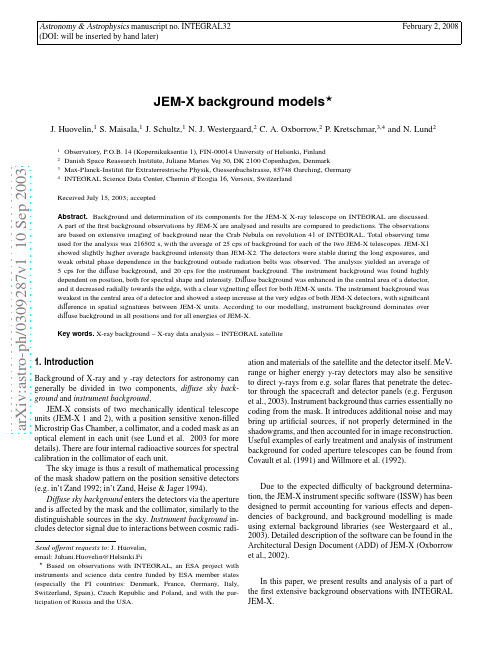
a r X i v :a s t r o -p h /0309287v 1 10 S e p 2003Astronomy &Astrophysics manuscript no.INTEGRAL32February 2,2008(DOI:will be inserted by hand later)JEM-X background models ⋆J.Huovelin,1S.Maisala,1J.Schultz,1N.J.Westergaard,2C.A.Oxborrow,2P.Kretschmar,3,4and N.Lund 21Observatory,P.O.B.14(Kopernikuksentie 1),FIN-00014University of Helsinki,Finland 2Danish Space Reasearch Institute,Juliane Maries Vej 30,DK 2100Copenhagen,Denmark 3Max-Planck-Institut f¨u r Extraterrestrische Physik,Giessenbachstrasse,85748Garching,Germany 4INTEGRAL Science Data Center,Chemin d’Ecogia 16,Versoix,Switzerland Received July 15,2003;accepted Abstract.Background and determination of its components for the JEM-X X-ray telescope on INTEGRAL are discussed.A part of the first background observations by JEM-X are analysed and results are compared to predictions.The observations are based on extensive imaging of background near the Crab Nebula on revolution 41of INTEGRAL.Total observing time used for the analysis was 216502s,with the average of 25cps of background for each of the two JEM-X telescopes.JEM-X1showed slightly higher average background intensity than JEM-X2.The detectors were stable during the long exposures,and weak orbital phase dependence in the background outside radiation belts was observed.The analysis yielded an average of 5cps for the di ffuse background,and 20cps for the instrument background.The instrument background was found highly dependent on position,both for spectral shape and intensity.Di ffuse background was enhanced in the central area of a detector,and it decreased radially towards the edge,with a clear vignetting e ffect for both JEM-X units.The instrument background was weakest in the central area of a detector and showed a steep increase at the very edges of both JEM-X detectors,with significant di fference in spatial signatures between JEM-X units.According to our modelling,instrument background dominates over di ffuse background in all positions and for all energies of JEM-X.Key words.X-ray background –X-ray data analysis –INTEGRAL satellite 1.Introduction Background of X-ray and γ-ray detectors for astronomy can generally be divided in two components,di ffuse sky back-ground and instrument background .JEM-X consists of two mechanically identical telescope units (JEM-X 1and 2),with a position sensitive xenon-filledMicrostrip Gas Chamber,a collimator,and a coded mask as anoptical element in each unit (see Lund et al.2003for moredetails).There are four internal radioactive sources for spectralcalibration in the collimator of each unit.The sky image is thus a result of mathematical processingof the mask shadow pattern on the position sensitive detectors(e.g.in’t Zand 1992;in’t Zand,Heise &Jager 1994).Di ffuse sky background enters the detectors via the apertureand is a ffected by the mask and the collimator,similarly to thedistinguishable sources in the sky.Instrument background in-cludes detector signal due to interactions between cosmic radi-2Huovelin et al.:JEM-X background modelsFig.1.Spatial distribution of the background.Upper panels:JEM-X1,lower panels,JEM-X2.Left panels:Instrument back-ground,Right panels:Diffuse background.The white rectan-gles denote the positions of the calibration sources,which havebeen excluded from our analysis.The collimator signature canbe seen as weak vertical and horizontal line structures in the shadowgrams.The broad vertical lines are due to dead anodes.Also some photon leak from the calibration sources is evident.The sharp and very narrow lines are graphical artifacts causedby the plotting routine.Total intensity of each shadowgram isnormalized to1.Table1.INTEGRAL background pointings during cycle41.45324.0+210850.17000053645.0+122415.14082553645.2+122546.44277553645.3+122543.564468Huovelin et al.:JEM-X background models3Table2.The normalization factors of the background con-tinuum components(10−3photons keV−1cm−2s−1at1keV). Mean and standard deviation of values derived from the six extraction regions at each radius are given.The energy range used in thefitting is4-33keV.Diffuse denotes diffuse sky back-ground,Flat denotes theflat continuum of the instrument back-ground.Note that the normalization is determined on the basis of source spectra from1R in R out JEM-X1JEM-X2pix pix Diffuse Flat Diffuse FlatThe diffuse background decreases towards the edges of the detector,as expected.The instrument background is stronger than expected,dominating the spectrum at all radii.The ten expected K-shell lines(from the109Cd and55Fe calibration sources,collimator(Mo),and detector gas(Xe))were detected close to their nominal positions.This implies that the energy scale is correctly determined.The previously unknown weak line near13keV turned out to be the uranium L-shell line.It most likely originates in the detector beryllium window.Near the edges of the detector,the background is highly nonuniform. Additional nonuniformity in the outer parts was introduced by photon leak from calibration sources,which could not be com-pletely eliminated.We also searched for possible dependence of background on the orbital phase of the observations.The spectrum varied with a range of approximately5%between three separate or-bital sections well outside radiation belts.The variation is sta-tistically significant but small.Also dependence on solar aspect angle and particle radiation level can be utilised in the JEM-X ISSW background modelling.Significant variations were not found.The variation in the solar aspect due to different point-ings was20◦,which is probably not sufficiently large for stud-ies of an effect on instrument background.Also,there was no proper indicator of particle radiation level on INTEGRAL available during our observations to search for a correlation.4.ConclusionsWe have analyzed a part of thefirst INTEGRAL background observations with JEM-X.Estimates of the spatial and spec-tral distributions are obtained for diffuse sky background and instrument background.The total background observed for JEM-X1was28cps,for JEM-X223cps,and25cps on the average.A part(∼1/5)of the excessively large background may be due to residual Crab Nebula emission in JEM-X data.According to XSPECfitting,the diffuse background was at maximum in the centre of the detector and it decreasedra-Fig.2.Four sample background spectra extracted from differ-ent parts of JEM-X2.At the sides of the detector,a blend of K-shell lines from the spacecraft structure is seen.Note also the prominent lines in spectrum extracted from the surround-ings of the calibrationsources.Fig.3.The background extraction regions.Units in both axes are pixels.All regions cover an equal area of the detector. Exclusion of calibration sources(not shown)reduces the ac-tual area of some regions.dially towards the edge,which is due to vignetting.There is also slight asymmmetry in the spatial distribution of the diffuse background,which is caused by a small angular misalignment of the detector plane.The count rate for diffuse background was approximately20%of the total background.The instrument background intensity and spectrum are highly position dependent,with a steep increase near the edges at all radial directions.Leakage of the radiative calibration sources causes residual line emission in the neighbourhood of4Huovelin et al.:JEM-X background modelsTable3.The lines detected from the background.Line ID is the element and transitions producing the line,E is the line en-ergy in keV(Thompson et al.,2001).Subscripts1and2denote the detectors JEM-X1and2,F is the largest line strength de-tected,¯F(N)mean of detected line strengths where N is the number of regions from which the line is detected(maximum is48regions/detector).The Mn/Fe line at6.45keV is a blend of Mn Kβ(6.49keV)and Fe Kα(6.40keV).Line strengths are given in10−3photons cm−2s−1.Note that the line strengths are determined on the basis of source spectra from1Line E F1¯F1(N)F2¯F2(N)Origin the source positions.The count rate for the instrument back-ground was approximately80%of the total background.The total background level varied with a range of approx-imately5%between different orbital sections.the variation is significant,but small.Also,it is impossible to say,what fraction of this,if any,is caused by the simultaneous variation of the so-lar aspect angle of the satellite,and the unknown variations of particle radiation level.We plan to separate these effects by the support of future background observations.Although our modelling is simple,and does not provide accurate absolute estimates of physical backgroundfluxes,it yields information which can be applied to the JEM-X analysis software to properly account for background contribution in spatially resolved spectral data.A thorough analysis of JEM-X background will be presented in a future paper. Acknowledgements.Authors from the Observatory,University of Helsinki acknowledge the Academy of Finland,TEKES,and the Finnish space research programme ANTARES forfinancial support in this research.J.Schultz is grateful for thefinancial support of the Wihuri Foundation.The Danish Space Research Institute acknowl-edges support given to the development of the JEM-X instrument from the PRODEX programme.ReferencesArnaud,K.A.,1996,Astronomical Data Analysis Software and Systems V,eds.Jacoby G.and Barnes J.,ASP Conf.Series V ol.101.Covault,C.E.,Grindlay,J.E.,Manandhar,R.P.,and Braga,J.,1991, IEEE Transact.Nucl.Sci.,V ol.38,No.2.Ferguson,C.,Barlow,E.J.,Bird,A.J.,et al.,2003A&A,this volume in’t Zand,J.,1992,Ph.D.thesis,SRON.in’t Zand,J.,Heise,J.,Jager,R.,1994,A&A288,665.Lund,.N.,Brandt,S.,Budtz-Joergensen,C.,et al.,2003,A&A,this volumeMarshall,F.E.,Boldt,E.A.,Holt,S.S.,et al.,1980,ApJ235,4 Oxborrow C.A.,Kretschmar,P.,Maisala,S.,Westergaard,N.J., Larsson,S.,2002,Instrument Specific Software for JEM-X: Architectural Design Document,DSRI homepage:www.dsri.dk Thompson, A.C.,Attwood, D.T.,Gullikson, E.M.,et al.,2001,“The X-ray data booklet”,2nd ed.,Lawrence Berkley National Laboratory,Univ.of California,available at / Westergaard,N.J.,Kretschmar,P.,Oxborrow,C.A.,et al.,2003,A& A,this volumeWillmore,A.P.,Bertram,D.,Watt,M.P.,et al.,1992,MNRAS258, 621。

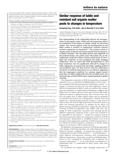
spectrometer equipped with a automatic carbonate preparation system(CAPS).Results are reported relative to the Vienna Pee Dee Belemnite standard(VPDB).Standard external analytical precision,based on replicate analysis of in-house standards calibrated to NBS-19,is better than0.1‰for d18O and d13C.Received1September;accepted25October2004;doi:10.1038/nature03135.1.Broecker,W.S.&Peng,T.-H.The role of CaCO3compensation in the glacial to interglacialatmospheric CO2change.Glob.Biogeochem.Cycles1,15–29(1987).2.Van Andel,T.H.Mesozoic/Cenozoic calcite compensation depth and the global distribution ofcalcareous sediments.Earth Planet.Sci.Lett.26,187–194(1975).3.Kennett,J.P.&Shackleton,N.J.Oxygen isotopic evidence for the development of the psychrosphere38Myr ago.Nature260,513–515(1976).ler,K.G.,Wright,J.D.&Fairbanks,R.G.Unlocking the ice house:Oligocene-Miocene oxygenisotopes,eustasy,and margin erosion.J.Geophys.Res.96,B4,6829–6849(1991).5.Zachos,J.C.,Quinn,T.M.&Salamy,K.A.High-resolution(104years)deep-sea foraminiferal stableisotope records of the Eocene-Oligocene climate transition.Palaeoceanography11,251–266(1996).6.Lear,C.H.,Elderfield,H.&Wilson,P.A.Cenozoic deep-sea temperatures and global ice volumesfrom Mg/Ca in benthic foraminiferal calcite.Science287,269–272(2000).7.DeConto,R.M.&Pollard,D.Rapid Cenozoic glaciation of Antarctica triggered by decliningatmospheric CO2.Nature421,245–249(2003).8.Shipboard Scientific Party2002.Leg199summary.Proc.ODP Init.Rep.(eds Lyle,M.W.,Wilson,P.A.&Janecek,T.R.)199,1–87(2002).skar,J.et al.Long term evolution and chaotic diffusion of the insolation quantities of Mars.Icarus170,343–364(2004).10.Peterson,L.C.Backman,te Cenozoic carbonate accumulation and the history of the carbonatecompensation depth in the western equatorial Indian Ocean.Proc.ODP Sci.Res.(eds Duncan,R.A., Backman,J.,Dunbar,R.B.&Peterson,L.C.)115,467–489(1990).11.Salamy,K.A.&Zachos,test Eocene-Early Oligocene climate change and Southern Oceanfertility:inferences from sediment accumulation and stable isotope data.Palaeogeogr.Palaeoclimatol.Palaeoecol.145,61–77(1999).12.Ehrmann,W.U.&Mackensen,A.Sedimentological evidence for the formation of an East Antarcticice sheet in Eocene/Oligocene time.Palaeogeogr.Palaeoclimatol.Palaeoecol.93,85–112(1992). 13.Ivany,L.C.,Patterson,W.P.&Lohmann,K.C.Cooler winters as a possible cause of mass extinction atthe Eocene/Oligocene boundary.Nature407,887–890(2000).14.Pa¨like,H.,Laskar,J.&Shackleton,N.J.Geologic constraints on the chaotic diffusion of the solarsystem.Geology32(11),929–932doi:10.1130/G20750(2004).15.Billups,K.&Schrag,D.P.Application of benthic foraminiferal Mg/Ca ratios to questions of Cenozoicclimate change.Earth Planet.Sci.Lett.209,181–195(2003).16.Lear,C.H.,Rosenthal,Y.,Coxall,H.K.&Wilson,te Eocene to early Miocene ice-sheetdynamics and the global carbon cycle.Paleoceanography19,doi:10.1029/2004PA001039(2004). 17.Pekar,S.F.,Christie-Blick,N.,Kominz,M.A.&Miller,K.G.Calibration between eustatic estimatesfrom backstripping and oxygen isotopic records for the Oligocene.Geology30,903–906(2002). 18.Lythe,M.B.,Vaughan,D.G.&BEDMAP Consortium,BEDMAP:A new ice thickness and subglacialtopographic model of Antarctica.J.Geophys.Res.106,B6,11335–11351(2001).19.Huybrechts,P.Sea-level changes at the LGM from ice-dynamic reconstructions of the Greenland andAntarctic ice sheets during the glacial cycles.Quat.Sci.Rev.21,203–231(2002).20.Hindmarsh,R.C.A.Time-scales and degrees of freedom operating in the evolution of continental ice-sheets.Trans.R.Soc.Edinb.Earth Sci.81,371–384(1990).21.Davies,R.,Cartwright,J.,Pike,J.&Line,C.Early Oligocene initiation of North Atlantic deep waterformation.Nature410,917–920(2001).22.Archer,D.&Maier-Reimer,E.Effect of deep-sea sedimentary calcite preservation on atmosphericCO2concentration.Nature367,260–263(1994).23.Sigman,D.M.&Boyle,E.A.Glacial/interglacial variations in atmospheric carbon dioxide.Nature407,859–869(2000).24.Zeebe,R.E.&Westbroek,P.A simple model for the CaCO3saturation state of the ocean:The“Strangelove,”the“Neritan,”and the“Cretan”Ocean.Geochem.Geophys.Geosyst.4,1104(2003).25.Kump,L.R.&Arthur,M.A.in Tectonics Uplift and Climate Change(ed.Ruddiman,W.F.)399–426(Plenum,New York,1997).26.Zachos,J.C.,Opdyke,B.N.,Quinn,T.M.,Jones,C.E.&Halliday,A.N.Early Cenozoic glaciation,Antarctic weathering and seawater87Sr/86Sr;is there a link?Chem.Geol.161,165–180(1999). 27.Ravizza,G.&Peucker-Ehrenbrink,B.The marine187Os/188Os record of the Eocene-Oligocenetransition:the interplay of weathering and glaciation.Earth Planet.Sci.Lett.210,151–165(2003).28.Berger,W.H.&Winterer,E.L.in Plate Stratigraphy and the Fluctuating Carbonate line in PelagicSediments:On Land and Under the Sea(eds Hsu¨,K.J.&Jenkyns,H.C.)11–48(Int.Assoc.Sedimentologists Spec.Publ.1,Blackwell Science,Oxford,1974).29.Opdyke,B.N.&Wilkinson,B.H.Surface area control of shallow cratonic to deep marine carbonateaccumulation.Paleoceanography3,685–703(1989).30.Harrison,K.G.Role of increased marine silica input on paleo-pCO2levels.Paleoceanography15,292–298(2000).Supplementary Information accompanies the paper on /nature. Acknowledgements We thank the Shipboard Party of Ocean Drilling Program Leg199for assistance at sea and M.Bolshaw,M.Cooper and H.Birch for laboratory assistance.This work was supported by a NERC UK ODP grant to P.A.W.,a Royal Commission for the Exhibition of1851 fellowship awarded to H.K.C.and by Swedish Research Council(VR)funding to H.P.We thank W.Broecker,R.Hindmarsh,S.D’Hondt,A.Merico,Y.Rosenthal,R.Rickaby,J.Shepherd and T.Tyrrell for discussions and comments on an earlier draft and L.Kump for a constructive review.Competing interests statement The authors declare that they have no competingfinancial interests.Correspondence and requests for materials should be addressed to P.A.W.(paw1@)............................................................... Similar response of labile and resistant soil organic matterpools to changes in temperature Changming Fang1,Pete Smith1,John B.Moncrieff2&Jo U.Smith11School of Biological Sciences,University of Aberdeen,Aberdeen AB243UU,UK 2Ecology and Resource Management,School of GeoSciences,The University of Edinburgh,Edinburgh EH93JU,UK ............................................................................................................................................................................. Our understanding of the relationship between the decompo-sition of soil organic matter(SOM)and soil temperature affects our predictions of the impact of climate change on soil-stored carbon1.One current opinion is that the decomposition of soil labile carbon is sensitive to temperature variation whereas resistant components are insensitive2–4.The resistant carbon or organic matter in mineral soil is then assumed to be unresponsive to global warming2,4.But the global pattern and magnitude of the predicted future soil carbon stock will mainly rely on the temperature sensitivity of these resistant carbon pools.To inves-tigate this sensitivity,we have incubated soils under changing temperature.Here we report that SOM decomposition or soil basal respiration rate was significantly affected by changes in SOM components associated with soil depth,sampling method and incubation time.Wefind,however,that the temperature sensitivity for SOM decomposition was not affected,suggesting that the temperature sensitivity for resistant organic matter pools does not differ significantly from that of labile pools,and that both types of SOM will therefore respond similarly to global warming.The temperature sensitivity of SOM decomposition,commonly referred to as Q10,is critical for modelling changes in soil C stock3–6. The assumption that the decomposition of old organic matter2–3or organic C in mineral soil4does not vary with temperature—that is, that the decomposition of labile C pools are sensitive,but resistant pools are insensitive,to temperature perturbations—suggests that higher losses of carbon will occur from soils in boreal and tundra regions in response to global warming.This is because these soils have the largest store of labile organic matter,and are predicted to experience the greatest rise in temperature7.Tropical soils may release less C than previously predicted4owing to a large store of SOM in deep soil8and the high proportion of resistant C pools in SOM.Soil warming experiments,an analogue for the effects of global warming on SOM decomposition9,suggest that the effect of warming on SOM decomposition may decline with time.The change in SOM composition associated with warming and the different temperature sensitivity of the C pools were assumed to be responsible for this decline10–11.Despite the common assertion that SOM composition affects the temperature sensitivity of SOM decomposition,experimental or modelling evidence is yet to be presented.If the temperature sensitivity of SOM decomposition is not affected by SOM composition,predictions of climate change impacts on soil stored C will be greatly affected.By definition,the temperature sensitivity of SOM decomposition is the change in SOM decomposition rate with temperature under otherwise constant conditions5.At present,this concept is often confused with concepts of SOM turnover4,12–13or SOM dynamics2–4 under different environmental conditions with accompanying different temperatures.Temperature sensitivity of SOM decompo-sition(or Q10)estimated by incubating soils at different but constant temperatures14–16or by radiocarbon accumulation in undisturbed soils13is confounded by many factors other than temperature.We incubated soil samples under changing temperature toletters to natureNATURE|VOL433|6JANUARY2005|/nature57©2005Nature Publishing Groupinvestigate the influence of SOM composition on the temperature dependence of SOM decomposition.Figure 1shows that soil C contents for both labile components (water-dissolved organic carbon (DOC),microbial carbon (C mic )and K 2SO 4-extracted carbon (C KSO ))and the total organic carbon (TOC),are signifi-cantly lower in the subsoil (20–30cm)than in the surface soil (0–10cm).The ratio of DOC:TOC and C KSO :TOC declined signifi-cantly with soil depth (F ¼28.5and 36.1,respectively,P ,0.0001),but C mic :TOC was not significantly affected by depth (F ¼1.9,P ,0.2).After the initial flush of CO 2emission,soil basal respi-ration rate at 208C was (mean ^s.e.m.)6.67^0.46m g CO 2per g dry soil per h for root-free samples in the 0–10cm layer,but only 1.92^0.20m g CO 2per g dry soil per h for the 20–30cm layer.Corresponding values were 6.27^0.66and 1.47^0.16for intact samples.Over a period up to 88days,the subsoil respired only ,0.29^0.13of the CO 2respired in the surface soil.These results indicate that soil basal respiration rate is closely related to variations in C pools occurring at different soil depths.Q 10values for individual soil samples varied in the range 1.97–2.21during the early stage of incubation (up to day 10).No significant correlation was found between Q 10and the rate of basal respiration.Relationships in Fig.1between respiration rate,Q 10value and SOM pools reflect the long-term acclimation of the microbial community to the environment (such as temperature,moisture and O 2)associated with soil depths.During the incubation,there was a significant decline in the labile components (Fig.2c,d,f).After 108days incubation,DOC was 0.73^0.14and C KSO was 0.62^0.065of initial values when averaged over all samples.The greatest variation following incu-bation was observed in C mic .The average C mic at day 42was only 0.43^0.13of the initial content,and less than 0.10^0.0057after 108days incubation.Changes in the average TOC during incu-bation were not significant (Fig.2b).At the end of the incubation,average TOC was 0.94^0.19of the initial content.Soil respiration rate consistently declined with time (Fig.2e).The association between respiration rate and C mic during the incubation suggests that the variation in microbial biomass may be a major cause of the temporal changes in soil respiration.The response of soil basal respiration to temperature was notaffected by the depletion of labile C during the incubation.Q 10values averaged for all samples were in the range 2.01–2.30for the whole incubation period (Fig.2a).There is no significant change in Q 10for soil basal respiration with incubation time,despite the fact that Q 10was more variable during the later stages of incubation.As time progressed,the resistant C component contributed a greater portion of the total soil basal respiration owing to the depletion of labile C pools (Supplementary Fig.2).The Q 10value for soil basal respiration should gradually decrease if resistant C is significantly different from labile pools and insensitive to temperature variation (Supplementary Fig.3).A constant Q 10for soil basal respiration suggests that the temperature dependence of resistant C is not significantly different from that for labile pools.In most incubation experiments,soil samples have been sepa-rately incubated at different but constant temperatures 12,14,15.Three different methods have been used to estimate SOM decomposition and its temperature sensitivity:the total mass loss 3,17,the time required for a given percentage of mass loss 17,and the soil respir-ation rate 14,18.A decline in soil respiration rate was commonly observed as incubation times increased 14,17,19,20.This decline is expected to be greater at higher than at lower temperatures because of the greater depletion and degradation of C pools 21.Temperature sensitivity is likely to be underestimated if turnover rate is derived from studies of total mass loss for a given time period or from respiration rates at different constant temperatures,owing to the higher decline in C turnover rate at higher temperature.If Q 10is estimated using the time required for a given percentage of mass loss,the value will be overestimated.In this case,temporal effects on estimated C turnover rate are more pronounced at lower temperatures than at higher temperatures.Data of total mass loss from soil incubations longer than one year were used to support the opinion that decomposition rates of organic matter in mineral soil do not vary with temperature 4.Estimated C turnover rates from a long-term incubation will be significantly different from those occurring in the field,owing to the quick decline in soil microbial biomass and respiration rate during incubation.In such exper-iments,the temperature sensitivity of SOM decomposition may have been seriously biased or underestimated because respiration rates at all temperatures are close to zero at the later stage of incubation.In soil warming experiments,the observed decline of warming effects on SOM decomposition with time 11does not necessarily mean that the decomposition of resistant C is less sensitive to elevated temperature than the labile component.Provided that the increase in net primary production (NPP)due to warming islessFigure 1Soil carbon components,respiration rate and associated Q 10values with respect to soil depth and sampling method (four replicates for each sample).Respiration rate was an average of data measured at 208C in days 3and 5.The Q 10value was estimated with soil respiration rates under changing temperature for the period of days 3–10.All values are normalized against that of surface root-free sample.Soil respiration rate is significantly related to concentrations of C pools owing to soil depth andsampling method,but Q 10does not change with respiration rate or C concentrations.Error bars indicate standard deviation.DOC,dissolved organic carbon;TOC,total organiccarbon.Figure 2Variations in respiration rate and soil carbon pools with increasing incubation time.Values are averages of all four samples,and normalized by initial values.a ,Q 10value;b ,TOC;c ,DOC;d ,K 2SO 4-extracted C;e ,respiration rate at 208C;and f ,microbial biomass C.Error bars are standard deviation.Respiration rate declined rapidly owing to the depletion of labile components (DOC,C KSO and C mic ),but the Q 10value of soil respiration remained unchanged.letters to natureNATURE |VOL 433|6JANUARY 2005|/nature58© 2005Nature Publishing Groupthan the increase in SOM decomposition rate,a decline in warming effect on SOM decomposition is always expected.In the long-term, the microbial community may become acclimated to warming with changed activities.The contribution of this acclimation is not yet clear.For long-term climate change,the response of the resistant pool of SOM plays a critical role in regulating soil C stocks.Given the predicted climate change in Europe in the next century,the greatest loss of SOM is expected in soils where the present mean annual temperature(MAT)is less than48C,and this net release of SOM will gradually decrease with MAT gradient(Fig.3a–c).(This predicted climate change is climate forcing according to the implementation by the Hadley Centre Climate Model(HadCM3) of the Intergovernmental Panel on Climate Change(IPCC)A1FI (world market–fossil fuel intensive)emission scenario22.)With a moderate change in the temperature sensitivity of the resistant C pool(humus pool of the Rothamsted Carbon Model23only),from Q10¼2.98to about2.58(at108C),sensitivity induced change will significantly reduce the net SOM release in temperate soils(present MAT.48C).By2100,the reduction in SOM loss could be up to 46%in arable soil,37%in grassland,and32%in forest for regions where the present MAT is greater than158C(Fig.3d).At the global scale,this reduction will be large enough to change our prediction of the magnitude and spatial pattern of SOM stocks in the future.Our study does not support the opinion that resistant C pools are significantly less responsive to temperature variation than labile C pools.A MethodsSoil samples(intact and root-free)were collected from a middle-aged plantation of Sitka spruce(Picea sitchensis)in Scotland(568370N,38480W).Mineral soils were collected from four locations in the site at depths of0–10,20–30cm.Root-free samples were made by sieving soil through a2mm mesh to remove plant detritus,root and gravel.For each depth,approximately600–800g soil was taken and packed into a chamber to the original bulk density.Intact soil samples(,10£10cm)were taken next to each root-free sample, following the method of ref.5.Soil samples were analysed to determine TOC24,DOC25and C KSO26.C mic was determined by fumigation extraction26.Samples(16in total)were incubated in the laboratory using a programmable water bath(developed in The University of Edinburgh,UK).Temperature was changed commonly between4and448C (continuously increased from the lowest to the highest with a step of48C and then decreased,reaching a new temperature within two hours).Each temperature was held for about9h.Before and after each round of temperature change,soils were kept at208C for a few days.Soil moisture contents were monitored and adjusted accordingly by adding water at the surface of the soil sample,and fresh air was continuously passed through each chamber during the incubation.Respired CO2was measured with an infrared gas analyser in differential mode,logged every second for7min for each chamber,but only the average over the last four minutes was used.The16chambers were measured sequentially,and four rounds of measurement were made before changing to another temperature.During each round of temperature change,the mean respiration rate at a given temperature was an average of values measured at that temperature when the temperature was increasing and decreasing(Supplementary Fig.1).Mean respiration rates at different temperatures werefitted with an exponential model5ðR¼a exp½ln Q10ðT=10Þ Þto calculate the Q10 value.More information about data analysis is included in the Supplementary Methods, which also explain how we assessed contributions of the resistant C pool to the total SOM decomposition and its Q10.Received30July;accepted22October2004;doi:10.1038/nature03138.1.Lenton,T.M.&Huntingford,C.Global terrestrial carbon storage and uncertainties in its temperaturesensitivity examined with a simple model.Glob.Change Biol.9,1333–1352(2003).2.Liski,J.,Ilvesniemi,H.,Ma¨kela¨,A.&Westman,C.J.CO2emissions from soil in response to climaticwarming are overestimated—The decomposition of old soil organic matter is tolerant of temperature.Ambio28,171–174(1999).3.Thornley,J.H.M.&Cannell,M.G.R.Soil carbon storage response to temperature:a hypothesis.Ann.Bot.87,591–598(2001).4.Giardina,C.P.&Ryan,M.G.Evidence that decomposition rates of organic carbon in mineral soil donot vary with temperature.Nature404,858–861(2000).5.Fang,C.&Moncrieff,J.B.The dependence of soil CO2efflux on temperature.Soil Biol.Biochem.33,155–165(2001).6.Sanderman,J.,Amundson,R.G.&Baldocchi,D.D.Application of eddy covariance measurements tothe temperature dependence of soil organic matter mean residence time.Glob.Biogeochem.Cycles17, doi:10.1029/2001GB001833(2003).7.Schlesinger,W.H.&Andrews,J.A.Soil respiration and the global carbon cycle.Biogeochemistry48,7–20(2000).8.Jobba´gy,E.G.&Jackson,R.B.The vertical distribution of soil organic carbon and its relation toclimate and vegetation.Ecol.Appl.10,423–436(2000).9.Rustad,L.E.et al.A meta-analysis of the response of soil respiration,net nitrogen mineralization,andaboveground plant growth to experimental ecosystem warming.Oecologia126,543–562(2001). 10.Peterjohn,W.T.,Melillo,J.M.&Bowles,S.T.Soil warming and trace gasfluxes:experimental designand preliminaryflux results.Oecologia93,18–24(1993).11.Peterjohn,W.T.et al.Response of trace gasfluxes and N availability to experimentally elevated soiltemperature.Ecol.Appl.4,617–625(1994).12.Dalias,P.,Anderson,J.M.,Bottner,P.&Couˆteaux,M.-M.T emperature responses of carbonmineralization in conifer forest soils from different regional climates incubated under standard laboratory conditions.Glob.Change Biol.6,181–192(2001).13.Trumbore,S.E.,Chadwick,O.A.&Amundson,R.Rapid exchange between soil carbon andatmospheric carbon dioxide driven by temperature change.Science272,393–396(1996).14.Winkler,J.P.,Cherry,R.S.&Schlesinger,W.H.The Q10relationship of microbial respiration in atemperate forest soil.Soil Biol.Biochem.28,1067–1072(1996).15.MacDonald,N.W.,Zak,D.R.&Pregitzer,K.S.Temperature effects on kinetics of microbialrespiration and net nitrogen and sulfur mineralization.Soil Sci.Soc.Am.J.59,233–240(1995). 16.Ross,D.J.&Tate,K.R.Microbial C and N,and respiratory activity,in litter and soil of a southernbeech(Nothofagus)forest:distribution and properties.Soil Biol.Biochem.25,477–483(1994). 17.Reichstein,M.,Bednorz,F.,Broll,G.&Ka¨tterer,T.T emperature dependence of carbon mineralisation:conclusions from a long-term incubation of subalpine soil samples.Soil Biol.Biochem.32,947–958 (2000).18.Fierer,N.,Allen,A.S.,Schimel,J.P.&Holden,P.A.Controls on microbial CO2production:acomparison of surface and subsurface soil horizon.Glob.Change Biol.9,1322–1332(2003).19.Lovell,R.D.&Jarvis,S.C.Soil microbial biomass and activity in soil from different grasslandmanagement treatments stored under controlled conditions.Soil Biol.Biochem.30,2077–2085 (1998).20.Lomander,A.,Ka¨tterer,T.&Andre´n,O.Carbon dioxide evolution from top-and subsoil as affected bymoisture and constant andfluctuating temperature.Soil Biol.Biochem.30,2017–2022(1998). 21.Grisi,B.,Grace,C.,Brookes,P.C.,Benedetti,A.&Dell’abate,M.T.Temperature effects on organicmatter and microbial biomass dynamics in temperate and tropical soils.Soil Biol.Biochem.30, 1309–1315(1998).22.IPCC.Special Report on Emissions Scenarios(Cambridge Univ.Press,Cambridge,UK,2000).23.Coleman,K.&Jenkinson,D.S.in Evaluation of Soil Organic Matter Models Using Existing Long-TermDatasets(eds Powlson,D.S.,Smith,P.&Smith,J.U.)237–246(NATO ASI Series I Vol.38,Springer, Heidelberg,1996).24.Allen,S.E.,Grimshaw,H.M.,Parkingson,J.A.&Quarmby,C.Chemical Analysis of EcologicalMaterials137–139(Blackwell Scientific,Oxford,1974).25.Martin-Olmedo,P.&Rees,R.M.Short-term N availability in response to dissolved organic-carbonfrom poultry manure,alone or in combination with cellulose.Biol.Fert.Soils29,386–393(1999).26.O¨hlinger,R.in Methods in Soil Biology(eds Schinner,F.et al.)56–58(Springer,Berlin,1995). Supplementary Information accompanies the paper on /nature. Acknowledgements We thank M.Wattenbarch and C.Zhang for assistance with the modelling. The pan-European modelling used data sets arising from the EU-funded ATEAM project. Competing interests statement The authors declare that they have no competingfinancial interests.Correspondence and requests for materials should be addressed to C.F.(c.fang@).Figure3Changes in soil C by2100for European soils.The baseline(solid lines in a–c)was from the original Roth-C model23projection(Q10¼2.98at108C for all C pools).Thetemperature sensitivity of humus was changed to80%of the original value(Q10¼2.58at108C,dashed lines in a–c).The loss of soil C is an average of all grid cells(21,976cellsat100£100resolution)according to present MAT.The percentage of net soil C loss withmodified Q10¼2.58for humus is relative to baseline decreases with MAT gradient(d).SOM,soil organic matter.letters to natureNATURE|VOL433|6JANUARY2005|/nature59©2005Nature Publishing Group。

Advances in Applied Mathematics 应用数学进展, 2022, 11(4), 1675-1682Published Online April 2022 in Hans. /journal/aamhttps:///10.12677/aam.2022.114182基于再分析资料ERA5计算对流层延迟精度分析袁炜*，张显云#，苏雷贵州大学矿业学院，贵州贵阳收稿日期：2022年3月14日；录用日期：2022年4月8日；发布日期：2022年4月18日摘要对流层延迟是GNSS导航定位的重要误差源，目前有多种方法可实现天顶对流层延迟(ZTD)的估算。

ERA5作为ECMWF发布的最新一代再分析产品，能够提供覆盖全球的高时空分辨率气象资料，据此可估算出高精度的ZTD。

然而，当前对ERA5对流层延迟产品精度评价的相关研究仍甚少。

本文以高精度的IGS对流层延迟产品为参考，在编程实现ERA5对流层延迟估算的基础上，对其精度进行了评价。

试验结果表明：相较于GPT2w-1S模型和GPT3-1S模型，由ERA5气象资料估算的ZTD产品具有更高的精度，均方根误差分别提高了27.53 mm和27.50 mm。

关键词ERA5，对流层延迟模型，Saastamoinen模型，GPT，气象参数Accuracy Analysis of Tropospheric DelayCalculation Based on Reanalysis Data ERA5Wei Yuan*, Xianyun Zhang#, Lei SuMining School of Guizhou University, Guiyang GuizhouReceived: Mar. 14th, 2022; accepted: Apr. 8th, 2022; published: Apr. 18th, 2022AbstractTropospheric delay is an important error source for GNSS navigation and positioning, and there are many methods to estimate the zenith tropospheric delay (ZTD). As the latest generation of*第一作者。

1 在Ansys中出现“Shape testing revealed that 450 of the 1500 new or modified elements violate shape warning limits.”，是什么原因造成的呢？单元网格质量不够好，尽量用规则化网格，或者再较为细密一点。

2 在Ansys中，用Area Fillet对两空间曲面进行倒角时出现以下错误：Area 6 offset could not fully converge to offset distance 10. Maximum error between the two surfaces is 1% of offset distance.请问这是什么错误？怎么解决？其中一个是圆柱接管表面，一个是碟形封头表面。

ansys的布尔操作能力比较弱。

如果一定要在ansys里面做的话，那么你试试看先对线进行倒角，然后由倒角后的线形成倒角的面。

建议最好用UG、PRO/E这类软件生成实体模型然后导入到ansys。

3 在Ansys中，出现错误“There are 21 small equation solver pivot terms。

”，是否是在建立接触contact时出现的错误？不是建立接触对的错误，一般是单元形状质量太差（例如有接近零度的锐角或者接近180度的钝角）造成small equation solver pivot terms4 在Ansys中，出现警告“SOLID45 wedges are recommended only in regions of relatively low stress gradients.”，是什么意思？"这只是一个警告，它告诉你：推荐SOLID45单元只用在应力梯度较低的区域。

它只是告诉你注意这个问题，如果应力梯度较高，则可能计算结果不可信。

"5 ansys向adams导的过程中，出现如下问题“There is not enough memory for the Sparse Matrix Solver to proceed.Please shut down other applications that may be running or increase the virtual memory on your system and return ANSYS.Memory currently allocated for the Sparse Matrix Solver=50MB.Memory currently required for the Sparse Matrix Solver to continue=25MB”，是什么原因造成的？不清楚你ansys导入adams过程中怎么还需要使用Sparse Matrix Solver（稀疏矩阵求解器）。

第60卷第1-2期2021年1月Vol.60No.1-2Jan.2021中山大学学报（自然科学版）ACTA SCIENTIARUM NATURALIUM UNIVERSITATIS SUNYATSENI天琴轨道与星座设计进展*张雪峰1，叶伯兵1，檀庄斌2，袁慧敏1，罗成健1，焦磊1，谷德峰1，丁延卫1，梅健伟11.“天琴计划”教育部重点实验室，中山大学天琴中心&物理与天文学院，天琴前沿科学中心，国家航天局引力波研究中心，广东珠海5190822.中山大学航空航天学院，广东深圳518000摘要：天琴计划预计将在地球10万km高度附近处的圆轨道上部署三颗无拖曳控制卫星，组成近似等边三角形星座，并利用高精度星间激光干涉链路来探测宇宙空间中mHz频段的低频引力波信号。

采用地球高轨是天琴计划的显著特征，如何行之有效地设计和利用地球轨道是天琴方案面临的重要问题。

本文将从星座构型稳定性优化、轨道面与轨道半径选取、地月系引力场干扰效应评估、阴影规避这四个方面介绍天琴轨道与星座设计的主要研究进展。

关键词：空间引力波探测；天琴计划；轨道设计；星座构型；空间环境效应中图分类号：O412.1；P111；V412.4文献标志码：A文章编号：0529-6579（2021）01-0123-06 Orbit and constellation design for TianQin：progress reviewZHANG Xuefeng1，YE Bobing1，TAN Zhuangbin2，YUAN Huimin1，LUO Chengjian1，JIAO Lei1，GU Defeng1，DING Yanwei1，MEI Jianwei11.MOE Key Laboratory of TianQin Mission，TianQin Research Center for Gravitational Physics&Schoolof Physics and Astronomy，Frontiers Science Center for TianQin，CNSA Research Center for Gravita⁃tional Waves，Sun Yat-sen University（Zhuhai Campus），Zhuhai519082，China2.School of Aeronautics and Astronautics，Sun Yat-sen University（Shenzhen Campus），Shenzhen518000，ChinaAbstract：The TianQin project plans to deploy three drag-free controlled satellites in circular high Earth orbits at an altitude of105km.The satellites form a nearly equilateral-triangle constellation，and ex⁃change high-precision laser interferometric links to detect low-frequency gravitational waves in the mHz frequency band.TianQin features a geocentric concept，and is facing the challenge of designing and uti⁃lizing high Earth orbits to the best effect.In this paper，we briefly summarize the main progresses on TianQin’s orbit and constellation design，including constellation stability optimization，orbital orienta⁃tion and radius selection，the Earth-Moon’s gravity disturbance evaluation，and eclipse avoidance.Key words：space-based gravitational wave detection；TianQin project；orbit design；constellation con⁃figuration；space environmental effectDOI：10.13471/ki.acta.snus.2020.11.02.2020B112*收稿日期：2020-11-02录用日期：2020-11-18网络首发日期：2021-01-08基金项目：广东省基础与应用基础重大项目（2019B030302001）；国家自然科学基金（11805287）作者简介：张雪峰（1983年生），男；研究方向：空间引力波探测方案概念性研究、引力理论；E-mail：zhangxf38@；叶伯兵（1993年生），男；研究方向：天琴轨道设计与优化；E-mail：yebb3@（以上两位作者为共同第一作者）第60卷中山大学学报（自然科学版）1引言2016年初地面引力波探测LIGO团队宣布首次探测到了引力波［1］，这一重大突破使得人类能够用全新的手段观测宇宙，开启了引力波天文学的时代。

大气科学系微机应用基础Primer of microcomputer applicationFORTRAN77程序设计FORTRAN77 Program Design大气科学概论An Introduction to Atmospheric Science大气探测学基础Atmospheric Sounding流体力学Fluid Dynamics天气学Synoptic Meteorology天气分析预报实验Forecast and Synoptic analysis生产实习Daily weather forecasting现代气候学基础An introduction to modern climatology卫星气象学Satellite meteorologyC语言程序设计 C Programming大气探测实验Experiment on Atmospheric Detective Technique云雾物理学Physics of Clouds and fogs动力气象学Dynamic Meteorology计算方法Calculation Method诊断分析Diagnostic Analysis中尺度气象学Meso-Microscale Synoptic Meteorology边界层气象学Boundary Layer Meteorology雷达气象学Radar Meteorology数值天气预报Numerical Weather Prediction气象统计预报Meteorological Statical Prediction大气科学中的数学方法Mathematical Methods in Atmospheric Sciences专题讲座Seminar专业英语English for Meteorological Field of Study计算机图形基础Basic of computer graphics气象业务自动化Automatic Weather Service空气污染预测与防治Prediction and Control for Air Pollution现代大气探测Advanced Atmospheric Sounding数字电子技术基础Basic of Digital Electronic Techniqul大气遥感Remote Sensing of Atmosphere模拟电子技术基础Analog Electron Technical Base大气化学Atmospheric Chemistry航空气象学Areameteorology计算机程序设计Computer Program Design数值预报模式与数值模拟Numerical Model and Numerical Simulation接口技术在大气科学中的应用Technology of Interface in Atmosphere Sciences Application海洋气象学Oceanic Meteorology现代实时天气预报技术（MICAPS系统）Advanced Short-range Weather Forecasting Technique(MICAPS system)1) atmospheric precipitation大气降水2) atmosphere science大气科学3) atmosphere大气1.The monitoring and study of atmosphere characteristics in near space as an environment forspace weapon equipments and system have been regarded more important for battle support.随着临近空间飞行器的不断发展和运用,作为武器装备和系统环境的临近空间大气特性成为作战保障的重要条件。

Quasi-Normal Modes of Stars and Black HolesKostas D.KokkotasDepartment of Physics,Aristotle University of Thessaloniki,Thessaloniki54006,Greece.kokkotas@astro.auth.grhttp://www.astro.auth.gr/˜kokkotasandBernd G.SchmidtMax Planck Institute for Gravitational Physics,Albert Einstein Institute,D-14476Golm,Germany.bernd@aei-potsdam.mpg.dePublished16September1999/Articles/Volume2/1999-2kokkotasLiving Reviews in RelativityPublished by the Max Planck Institute for Gravitational PhysicsAlbert Einstein Institute,GermanyAbstractPerturbations of stars and black holes have been one of the main topics of relativistic astrophysics for the last few decades.They are of partic-ular importance today,because of their relevance to gravitational waveastronomy.In this review we present the theory of quasi-normal modes ofcompact objects from both the mathematical and astrophysical points ofview.The discussion includes perturbations of black holes(Schwarzschild,Reissner-Nordstr¨o m,Kerr and Kerr-Newman)and relativistic stars(non-rotating and slowly-rotating).The properties of the various families ofquasi-normal modes are described,and numerical techniques for calculat-ing quasi-normal modes reviewed.The successes,as well as the limits,of perturbation theory are presented,and its role in the emerging era ofnumerical relativity and supercomputers is discussed.c 1999Max-Planck-Gesellschaft and the authors.Further information on copyright is given at /Info/Copyright/.For permission to reproduce the article please contact livrev@aei-potsdam.mpg.de.Article AmendmentsOn author request a Living Reviews article can be amended to include errata and small additions to ensure that the most accurate and up-to-date infor-mation possible is provided.For detailed documentation of amendments, please go to the article’s online version at/Articles/Volume2/1999-2kokkotas/. Owing to the fact that a Living Reviews article can evolve over time,we recommend to cite the article as follows:Kokkotas,K.D.,and Schmidt,B.G.,“Quasi-Normal Modes of Stars and Black Holes”,Living Rev.Relativity,2,(1999),2.[Online Article]:cited on<date>, /Articles/Volume2/1999-2kokkotas/. The date in’cited on<date>’then uniquely identifies the version of the article you are referring to.3Quasi-Normal Modes of Stars and Black HolesContents1Introduction4 2Normal Modes–Quasi-Normal Modes–Resonances7 3Quasi-Normal Modes of Black Holes123.1Schwarzschild Black Holes (12)3.2Kerr Black Holes (17)3.3Stability and Completeness of Quasi-Normal Modes (20)4Quasi-Normal Modes of Relativistic Stars234.1Stellar Pulsations:The Theoretical Minimum (23)4.2Mode Analysis (26)4.2.1Families of Fluid Modes (26)4.2.2Families of Spacetime or w-Modes (30)4.3Stability (31)5Excitation and Detection of QNMs325.1Studies of Black Hole QNM Excitation (33)5.2Studies of Stellar QNM Excitation (34)5.3Detection of the QNM Ringing (37)5.4Parameter Estimation (39)6Numerical Techniques426.1Black Holes (42)6.1.1Evolving the Time Dependent Wave Equation (42)6.1.2Integration of the Time Independent Wave Equation (43)6.1.3WKB Methods (44)6.1.4The Method of Continued Fractions (44)6.2Relativistic Stars (45)7Where Are We Going?487.1Synergism Between Perturbation Theory and Numerical Relativity487.2Second Order Perturbations (48)7.3Mode Calculations (49)7.4The Detectors (49)8Acknowledgments50 9Appendix:Schr¨o dinger Equation Versus Wave Equation51Living Reviews in Relativity(1999-2)K.D.Kokkotas and B.G.Schmidt41IntroductionHelioseismology and asteroseismology are well known terms in classical astro-physics.From the beginning of the century the variability of Cepheids has been used for the accurate measurement of cosmic distances,while the variability of a number of stellar objects(RR Lyrae,Mira)has been associated with stel-lar oscillations.Observations of solar oscillations(with thousands of nonradial modes)have also revealed a wealth of information about the internal structure of the Sun[204].Practically every stellar object oscillates radially or nonradi-ally,and although there is great difficulty in observing such oscillations there are already results for various types of stars(O,B,...).All these types of pulsations of normal main sequence stars can be studied via Newtonian theory and they are of no importance for the forthcoming era of gravitational wave astronomy.The gravitational waves emitted by these stars are extremely weak and have very low frequencies(cf.for a discussion of the sun[70],and an im-portant new measurement of the sun’s quadrupole moment and its application in the measurement of the anomalous precession of Mercury’s perihelion[163]). This is not the case when we consider very compact stellar objects i.e.neutron stars and black holes.Their oscillations,produced mainly during the formation phase,can be strong enough to be detected by the gravitational wave detectors (LIGO,VIRGO,GEO600,SPHERE)which are under construction.In the framework of general relativity(GR)quasi-normal modes(QNM) arise,as perturbations(electromagnetic or gravitational)of stellar or black hole spacetimes.Due to the emission of gravitational waves there are no normal mode oscillations but instead the frequencies become“quasi-normal”(complex), with the real part representing the actual frequency of the oscillation and the imaginary part representing the damping.In this review we shall discuss the oscillations of neutron stars and black holes.The natural way to study these oscillations is by considering the linearized Einstein equations.Nevertheless,there has been recent work on nonlinear black hole perturbations[101,102,103,104,100]while,as yet nothing is known for nonlinear stellar oscillations in general relativity.The study of black hole perturbations was initiated by the pioneering work of Regge and Wheeler[173]in the late50s and was continued by Zerilli[212]. The perturbations of relativistic stars in GR werefirst studied in the late60s by Kip Thorne and his collaborators[202,198,199,200].The initial aim of Regge and Wheeler was to study the stability of a black hole to small perturbations and they did not try to connect these perturbations to astrophysics.In con-trast,for the case of relativistic stars,Thorne’s aim was to extend the known properties of Newtonian oscillation theory to general relativity,and to estimate the frequencies and the energy radiated as gravitational waves.QNMs werefirst pointed out by Vishveshwara[207]in calculations of the scattering of gravitational waves by a Schwarzschild black hole,while Press[164] coined the term quasi-normal frequencies.QNM oscillations have been found in perturbation calculations of particles falling into Schwarzschild[73]and Kerr black holes[76,80]and in the collapse of a star to form a black hole[66,67,68]. Living Reviews in Relativity(1999-2)5Quasi-Normal Modes of Stars and Black Holes Numerical investigations of the fully nonlinear equations of general relativity have provided results which agree with the results of perturbation calculations;in particular numerical studies of the head-on collision of two black holes [30,29](cf.Figure 1)and gravitational collapse to a Kerr hole [191].Recently,Price,Pullin and collaborators [170,31,101,28]have pushed forward the agreement between full nonlinear numerical results and results from perturbation theory for the collision of two black holes.This proves the power of the perturbation approach even in highly nonlinear problems while at the same time indicating its limits.In the concluding remarks of their pioneering paper on nonradial oscillations of neutron stars Thorne and Campollataro [202]described it as “just a modest introduction to a story which promises to be long,complicated and fascinating ”.The story has undoubtedly proved to be intriguing,and many authors have contributed to our present understanding of the pulsations of both black holes and neutron stars.Thirty years after these prophetic words by Thorne and Campollataro hundreds of papers have been written in an attempt to understand the stability,the characteristic frequencies and the mechanisms of excitation of these oscillations.Their relevance to the emission of gravitational waves was always the basic underlying reason of each study.An account of all this work will be attempted in the next sections hoping that the interested reader will find this review useful both as a guide to the literature and as an inspiration for future work on the open problems of the field.020406080100Time (M ADM )-0.3-0.2-0.10.00.10.20.3(l =2) Z e r i l l i F u n c t i o n Numerical solutionQNM fit Figure 1:QNM ringing after the head-on collision of two unequal mass black holes [29].The continuous line corresponds to the full nonlinear numerical calculation while the dotted line is a fit to the fundamental and first overtone QNM.In the next section we attempt to give a mathematical definition of QNMs.Living Reviews in Relativity (1999-2)K.D.Kokkotas and B.G.Schmidt6 The third and fourth section will be devoted to the study of the black hole and stellar QNMs.In thefifth section we discuss the excitation and observation of QNMs andfinally in the sixth section we will mention the more significant numerical techniques used in the study of QNMs.Living Reviews in Relativity(1999-2)7Quasi-Normal Modes of Stars and Black Holes 2Normal Modes–Quasi-Normal Modes–Res-onancesBefore discussing quasi-normal modes it is useful to remember what normal modes are!Compact classical linear oscillating systems such asfinite strings,mem-branes,or cavitiesfilled with electromagnetic radiation have preferred time harmonic states of motion(ωis real):χn(t,x)=e iωn tχn(x),n=1,2,3...,(1) if dissipation is neglected.(We assumeχto be some complex valuedfield.) There is generally an infinite collection of such periodic solutions,and the“gen-eral solution”can be expressed as a superposition,χ(t,x)=∞n=1a n e iωn tχn(x),(2)of such normal modes.The simplest example is a string of length L which isfixed at its ends.All such systems can be described by systems of partial differential equations of the type(χmay be a vector)∂χ∂t=Aχ,(3)where A is a linear operator acting only on the spatial variables.Because of thefiniteness of the system the time evolution is only determined if some boundary conditions are prescribed.The search for solutions periodic in time leads to a boundary value problem in the spatial variables.In simple cases it is of the Sturm-Liouville type.The treatment of such boundary value problems for differential equations played an important role in the development of Hilbert space techniques.A Hilbert space is chosen such that the differential operator becomes sym-metric.Due to the boundary conditions dictated by the physical problem,A becomes a self-adjoint operator on the appropriate Hilbert space and has a pure point spectrum.The eigenfunctions and eigenvalues determine the periodic solutions(1).The definition of self-adjointness is rather subtle from a physicist’s point of view since fairly complicated“domain issues”play an essential role.(See[43] where a mathematical exposition for physicists is given.)The wave equation modeling thefinite string has solutions of various degrees of differentiability. To describe all“realistic situations”,clearly C∞functions should be sufficient. Sometimes it may,however,also be convenient to consider more general solu-tions.From the mathematical point of view the collection of all smooth functions is not a natural setting to study the wave equation because sequences of solutionsLiving Reviews in Relativity(1999-2)K.D.Kokkotas and B.G.Schmidt8 exist which converge to non-smooth solutions.To establish such powerful state-ments like(2)one has to study the equation on certain subsets of the Hilbert space of square integrable functions.For“nice”equations it usually happens that the eigenfunctions are in fact analytic.They can then be used to gen-erate,for example,all smooth solutions by a pointwise converging series(2). The key point is that we need some mathematical sophistication to obtain the “completeness property”of the eigenfunctions.This picture of“normal modes”changes when we consider“open systems”which can lose energy to infinity.The simplest case are waves on an infinite string.The general solution of this problem isχ(t,x)=A(t−x)+B(t+x)(4) with“arbitrary”functions A and B.Which solutions should we study?Since we have all solutions,this is not a serious question.In more general cases, however,in which the general solution is not known,we have to select a certain class of solutions which we consider as relevant for the physical problem.Let us consider for the following discussion,as an example,a wave equation with a potential on the real line,∂2∂t2χ+ −∂2∂x2+V(x)χ=0.(5)Cauchy dataχ(0,x),∂tχ(0,x)which have two derivatives determine a unique twice differentiable solution.No boundary condition is needed at infinity to determine the time evolution of the data!This can be established by fairly simple PDE theory[116].There exist solutions for which the support of thefields are spatially compact, or–the other extreme–solutions with infinite total energy for which thefields grow at spatial infinity in a quite arbitrary way!From the point of view of physics smooth solutions with spatially compact support should be the relevant class–who cares what happens near infinity! Again it turns out that mathematically it is more convenient to study all solu-tions offinite total energy.Then the relevant operator is again self-adjoint,but now its spectrum is purely“continuous”.There are no eigenfunctions which are square integrable.Only“improper eigenfunctions”like plane waves exist.This expresses the fact that wefind a solution of the form(1)for any realωand by forming appropriate superpositions one can construct solutions which are “almost eigenfunctions”.(In the case V(x)≡0these are wave packets formed from plane waves.)These solutions are the analogs of normal modes for infinite systems.Let us now turn to the discussion of“quasi-normal modes”which are concep-tually different to normal modes.To define quasi-normal modes let us consider the wave equation(5)for potentials with V≥0which vanish for|x|>x0.Then in this case all solutions determined by data of compact support are bounded: |χ(t,x)|<C.We can use Laplace transformation techniques to represent such Living Reviews in Relativity(1999-2)9Quasi-Normal Modes of Stars and Black Holes solutions.The Laplace transformˆχ(s,x)(s>0real)of a solutionχ(t,x)isˆχ(s,x)= ∞0e−stχ(t,x)dt,(6) and satisfies the ordinary differential equations2ˆχ−ˆχ +Vˆχ=+sχ(0,x)+∂tχ(0,x),(7) wheres2ˆχ−ˆχ +Vˆχ=0(8) is the homogeneous equation.The boundedness ofχimplies thatˆχis analytic for positive,real s,and has an analytic continuation onto the complex half plane Re(s)>0.Which solutionˆχof this inhomogeneous equation gives the unique solution in spacetime determined by the data?There is no arbitrariness;only one of the Green functions for the inhomogeneous equation is correct!All Green functions can be constructed by the following well known method. Choose any two linearly independent solutions of the homogeneous equation f−(s,x)and f+(s,x),and defineG(s,x,x )=1W(s)f−(s,x )f+(s,x)(x <x),f−(s,x)f+(s,x )(x >x),(9)where W(s)is the Wronskian of f−and f+.If we denote the inhomogeneity of(7)by j,a solution of(7)isˆχ(s,x)= ∞−∞G(s,x,x )j(s,x )dx .(10) We still have to select a unique pair of solutions f−,f+.Here the information that the solution in spacetime is bounded can be used.The definition of the Laplace transform implies thatˆχis bounded as a function of x.Because the potential V vanishes for|x|>x0,the solutions of the homogeneous equation(8) for|x|>x0aref=e±sx.(11) The following pair of solutionsf+=e−sx for x>x0,f−=e+sx for x<−x0,(12) which is linearly independent for Re(s)>0,gives the unique Green function which defines a bounded solution for j of compact support.Note that for Re(s)>0the solution f+is exponentially decaying for large x and f−is expo-nentially decaying for small x.For small x however,f+will be a linear com-bination a(s)e−sx+b(s)e sx which will in general grow exponentially.Similar behavior is found for f−.Living Reviews in Relativity(1999-2)K.D.Kokkotas and B.G.Schmidt 10Quasi-Normal mode frequencies s n can be defined as those complex numbers for whichf +(s n ,x )=c (s n )f −(s n ,x ),(13)that is the two functions become linearly dependent,the Wronskian vanishes and the Green function is singular!The corresponding solutions f +(s n ,x )are called quasi eigenfunctions.Are there such numbers s n ?From the boundedness of the solution in space-time we know that the unique Green function must exist for Re (s )>0.Hence f +,f −are linearly independent for those values of s .However,as solutions f +,f −of the homogeneous equation (8)they have a unique continuation to the complex s plane.In [35]it is shown that for positive potentials with compact support there is always a countable number of zeros of the Wronskian with Re (s )<0.What is the mathematical and physical significance of the quasi-normal fre-quencies s n and the corresponding quasi-normal functions f +?First of all we should note that because of Re (s )<0the function f +grows exponentially for small and large x !The corresponding spacetime solution e s n t f +(s n ,x )is therefore not a physically relevant solution,unlike the normal modes.If one studies the inverse Laplace transformation and expresses χas a com-plex line integral (a >0),χ(t,x )=12πi +∞−∞e (a +is )t ˆχ(a +is,x )ds,(14)one can deform the path of the complex integration and show that the late time behavior of solutions can be approximated in finite parts of the space by a finite sum of the form χ(t,x )∼N n =1a n e (αn +iβn )t f +(s n ,x ).(15)Here we assume that Re (s n +1)<Re (s n )<0,s n =αn +iβn .The approxi-mation ∼means that if we choose x 0,x 1, and t 0then there exists a constant C (t 0,x 0,x 1, )such that χ(t,x )−N n =1a n e (αn +iβn )t f +(s n ,x ) ≤Ce (−|αN +1|+ )t (16)holds for t >t 0,x 0<x <x 1, >0with C (t 0,x 0,x 1, )independent of t .The constants a n depend only on the data [35]!This implies in particular that all solutions defined by data of compact support decay exponentially in time on spatially bounded regions.The generic leading order decay is determined by the quasi-normal mode frequency with the largest real part s 1,i.e.slowest damping.On finite intervals and for late times the solution is approximated by a finite sum of quasi eigenfunctions (15).It is presently unclear whether one can strengthen (16)to a statement like (2),a pointwise expansion of the late time solution in terms of quasi-normal Living Reviews in Relativity (1999-2)11Quasi-Normal Modes of Stars and Black Holes modes.For one particular potential(P¨o schl-Teller)this has been shown by Beyer[42].Let us now consider the case where the potential is positive for all x,but decays near infinity as happens for example for the wave equation on the static Schwarzschild spacetime.Data of compact support determine again solutions which are bounded[117].Hence we can proceed as before.Thefirst new point concerns the definitions of f±.It can be shown that the homogeneous equation(8)has for each real positive s a unique solution f+(s,x)such that lim x→∞(e sx f+(s,x))=1holds and correspondingly for f−.These functions are uniquely determined,define the correct Green function and have analytic continuations onto the complex half plane Re(s)>0.It is however quite complicated to get a good representation of these func-tions.If the point at infinity is not a regular singular point,we do not even get converging series expansions for f±.(This is particularly serious for values of s with negative real part because we expect exponential growth in x).The next new feature is that the analyticity properties of f±in the complex s plane depend on the decay of the potential.To obtain information about analytic continuation,even use of analyticity properties of the potential in x is made!Branch cuts may occur.Nevertheless in a lot of cases an infinite number of quasi-normal mode frequencies exists.The fact that the potential never vanishes may,however,destroy the expo-nential decay in time of the solutions and therefore the essential properties of the quasi-normal modes.This probably happens if the potential decays slower than exponentially.There is,however,the following way out:Suppose you want to study a solution determined by data of compact support from t=0to some largefinite time t=T.Up to this time the solution is–because of domain of dependence properties–completely independent of the potential for sufficiently large x.Hence we may see an exponential decay of the form(15)in a time range t1<t<T.This is the behavior seen in numerical calculations.The situation is similar in the case ofα-decay in quantum mechanics.A comparison of quasi-normal modes of wave equations and resonances in quantum theory can be found in the appendix,see section9.Living Reviews in Relativity(1999-2)K.D.Kokkotas and B.G.Schmidt123Quasi-Normal Modes of Black HolesOne of the most interesting aspects of gravitational wave detection will be the connection with the existence of black holes[201].Although there are presently several indirect ways of identifying black holes in the universe,gravitational waves emitted by an oscillating black hole will carry a uniquefingerprint which would lead to the direct identification of their existence.As we mentioned earlier,gravitational radiation from black hole oscillations exhibits certain characteristic frequencies which are independent of the pro-cesses giving rise to these oscillations.These“quasi-normal”frequencies are directly connected to the parameters of the black hole(mass,charge and angu-lar momentum)and for stellar mass black holes are expected to be inside the bandwidth of the constructed gravitational wave detectors.The perturbations of a Schwarzschild black hole reduce to a simple wave equation which has been studied extensively.The wave equation for the case of a Reissner-Nordstr¨o m black hole is more or less similar to the Schwarzschild case,but for Kerr one has to solve a system of coupled wave equations(one for the radial part and one for the angular part).For this reason the Kerr case has been studied less thoroughly.Finally,in the case of Kerr-Newman black holes we face the problem that the perturbations cannot be separated in their angular and radial parts and thus apart from special cases[124]the problem has not been studied at all.3.1Schwarzschild Black HolesThe study of perturbations of Schwarzschild black holes assumes a small per-turbation hµνon a static spherically symmetric background metricds2=g0µνdxµdxν=−e v(r)dt2+eλ(r)dr2+r2 dθ2+sin2θdφ2 ,(17) with the perturbed metric having the formgµν=g0µν+hµν,(18) which leads to a variation of the Einstein equations i.e.δGµν=4πδTµν.(19) By assuming a decomposition into tensor spherical harmonics for each hµνof the formχ(t,r,θ,φ)= mχ m(r,t)r Y m(θ,φ),(20)the perturbation problem is reduced to a single wave equation,for the func-tionχ m(r,t)(which is a combination of the various components of hµν).It should be pointed out that equation(20)is an expansion for scalar quantities only.From the10independent components of the hµνonly h tt,h tr,and h rr transform as scalars under rotations.The h tθ,h tφ,h rθ,and h rφtransform asLiving Reviews in Relativity(1999-2)13Quasi-Normal Modes of Stars and Black Holes components of two-vectors under rotations and can be expanded in a series of vector spherical harmonics while the components hθθ,hθφ,and hφφtransform as components of a2×2tensor and can be expanded in a series of tensor spher-ical harmonics(see[202,212,152]for details).There are two classes of vector spherical harmonics(polar and axial)which are build out of combinations of the Levi-Civita volume form and the gradient operator acting on the scalar spherical harmonics.The difference between the two families is their parity. Under the parity operatorπa spherical harmonic with index transforms as (−1) ,the polar class of perturbations transform under parity in the same way, as(−1) ,and the axial perturbations as(−1) +11.Finally,since we are dealing with spherically symmetric spacetimes the solution will be independent of m, thus this subscript can be omitted.The radial component of a perturbation outside the event horizon satisfies the following wave equation,∂2∂t χ + −∂2∂r∗+V (r)χ =0,(21)where r∗is the“tortoise”radial coordinate defined byr∗=r+2M log(r/2M−1),(22) and M is the mass of the black hole.For“axial”perturbationsV (r)= 1−2M r ( +1)r+2σMr(23)is the effective potential or(as it is known in the literature)Regge-Wheeler potential[173],which is a single potential barrier with a peak around r=3M, which is the location of the unstable photon orbit.The form(23)is true even if we consider scalar or electromagnetic testfields as perturbations.The parameter σtakes the values1for scalar perturbations,0for electromagnetic perturbations, and−3for gravitational perturbations and can be expressed asσ=1−s2,where s=0,1,2is the spin of the perturbingfield.For“polar”perturbations the effective potential was derived by Zerilli[212]and has the form V (r)= 1−2M r 2n2(n+1)r3+6n2Mr2+18nM2r+18M3r3(nr+3M)2,(24)1In the literature the polar perturbations are also called even-parity because they are characterized by their behavior under parity operations as discussed earlier,and in the same way the axial perturbations are called odd-parity.We will stick to the polar/axial terminology since there is a confusion with the definition of the parity operation,the reason is that to most people,the words“even”and“odd”imply that a mode transforms underπas(−1)2n or(−1)2n+1respectively(for n some integer).However only the polar modes with even have even parity and only axial modes with even have odd parity.If is odd,then polar modes have odd parity and axial modes have even parity.Another terminology is to call the polar perturbations spheroidal and the axial ones toroidal.This definition is coming from the study of stellar pulsations in Newtonian theory and represents the type offluid motions that each type of perturbation induces.Since we are dealing both with stars and black holes we will stick to the polar/axial terminology.Living Reviews in Relativity(1999-2)K.D.Kokkotas and B.G.Schmidt14where2n=( −1)( +2).(25) Chandrasekhar[54]has shown that one can transform the equation(21)for “axial”modes to the corresponding one for“polar”modes via a transforma-tion involving differential operations.It can also be shown that both forms are connected to the Bardeen-Press[38]perturbation equation derived via the Newman-Penrose formalism.The potential V (r∗)decays exponentially near the horizon,r∗→−∞,and as r−2∗for r∗→+∞.From the form of equation(21)it is evident that the study of black hole perturbations will follow the footsteps of the theory outlined in section2.Kay and Wald[117]have shown that solutions with data of compact sup-port are bounded.Hence we know that the time independent Green function G(s,r∗,r ∗)is analytic for Re(s)>0.The essential difficulty is now to obtain the solutions f±(cf.equation(10))of the equations2ˆχ−ˆχ +Vˆχ=0,(26) (prime denotes differentiation with respect to r∗)which satisfy for real,positives:f+∼e−sr∗for r∗→∞,f−∼e+r∗x for r∗→−∞.(27) To determine the quasi-normal modes we need the analytic continuations of these functions.As the horizon(r∗→∞)is a regular singular point of(26),a representation of f−(r∗,s)as a converging series exists.For M=12it reads:f−(r,s)=(r−1)s∞n=0a n(s)(r−1)n.(28)The series converges for all complex s and|r−1|<1[162].(The analytic extension of f−is investigated in[115].)The result is that f−has an extension to the complex s plane with poles only at negative real integers.The representation of f+is more complicated:Because infinity is a singular point no power series expansion like(28)exists.A representation coming from the iteration of the defining integral equation is given by Jensen and Candelas[115],see also[159]. It turns out that the continuation of f+has a branch cut Re(s)≤0due to the decay r−2for large r[115].The most extensive mathematical investigation of quasi-normal modes of the Schwarzschild solution is contained in the paper by Bachelot and Motet-Bachelot[35].Here the existence of an infinite number of quasi-normal modes is demonstrated.Truncating the potential(23)to make it of compact support leads to the estimate(16).The decay of solutions in time is not exponential because of the weak decay of the potential for large r.At late times,the quasi-normal oscillations are swamped by the radiative tail[166,167].This tail radiation is of interest in its Living Reviews in Relativity(1999-2)。