matlab魔幻图型代码与成品

Matlab图形绘制技巧与实例展示一、介绍Matlab是一种功能强大的计算机软件，常用于科学计算和数据可视化分析。

其中，图形绘制是Matlab的一项重要功能，能够直观地展示数据和结果。

本文将探讨一些Matlab图形绘制的技巧，并通过实例展示其应用。

二、基础图形绘制Matlab提供了多种基础图形绘制函数，如plot、scatter、bar等。

这些函数可以用来绘制折线图、散点图、柱状图等常见图形。

例如我们可以使用plot函数绘制一个简单的折线图：```matlabx = 1:10;y = [1, 2, 3, 4, 5, 4, 3, 2, 1, 0];plot(x, y);```运行以上代码，就可以得到一个由点连接而成的折线图。

通过修改x和y的取值，可以得到不同形状和样式的折线图。

三、图形修饰在绘制图形时，我们通常需要添加标题、坐标轴标签、图例等进行修饰。

Matlab提供了相应的函数，如title、xlabel、ylabel、legend等。

下面是一个例子：```matlabx = 1:10;y = [1, 4, 9, 16, 25, 16, 9, 4, 1, 0];plot(x, y);title('Parabolic Curve');xlabel('X-axis');ylabel('Y-axis');legend('Curve');```执行以上代码，我们得到一个带有标题、坐标轴标签和图例的折线图。

四、子图绘制有时候，我们希望在一幅图中同时显示多个子图，以便比较它们之间的关系。

Matlab提供了subplot函数来实现这个功能。

下面是一个例子：```matlabx = 1:10;y1 = [1, 2, 3, 4, 5, 4, 3, 2, 1, 0];y2 = [0, 1, 0, 1, 0, 1, 0, 1, 0, 1];subplot(2, 1, 1);plot(x, y1);title('Subplot 1');subplot(2, 1, 2);plot(x, y2);title('Subplot 2');通过subplot函数，我们将一幅图分为两个子图，并在每个子图中绘制不同的折线图。

哈哈哈MATLAB显示正炫余炫图：plot(x,y1,'* r',x,y2,'o b')定义【0,2π】；t=0:pi/10:2*pi;定义函数文件：function [返回变量列表]=函数名（输入变量列表）顺序结构：选择结构1）if-else-end语句其格式为：if 逻辑表达式程序模块1；else程序模块2；End图片读取：%选择图片路径[filename, pathname] = ...uigetfile({'*.jpg';'*.bmp';'*.gif'},'选择图片');%合成路径+文件名str=[pathname,filename];%为什么pathname和filename要前面出现的位置相反才能运行呢？？？%读取图片im=imread(str);%使用图片axes(handles.axes1);%显示图片imshow(im);边缘检测：global imstr=get(hObject,'string');axes (handles.axes1);switch strcase ' 原图'imshow(im);case 'sobel'BW = edge(rgb2gray(im),'sobel');imshow(BW);case 'prewitt'BW = edge(rgb2gray(im),'prewitt');imshow(BW);case 'canny'BW = edge(rgb2gray(im),'canny');imshow(BW);Canny算子边缘定位精确性和抗噪声能力效果较好，是一个折中方案end;开闭运算：se=[1,1,1;1,1,1;1,1,1;1,1,1]; %Structuring ElementI=rgb2gray(im);imshow(I,[]);title('Original Image');I=double(I);[im_height,im_width]=size(I);[se_height,se_width]=size(se);halfheight=floor(se_height/2);halfwidth=floor(se_width/2);[se_origin]=floor((size(se)+1)/2);image_dilation=padarray(I,se_origin,0,'both'); %Image to be used for dilationimage_erosion=padarray(I,se_origin,256,'both'); %Image to be used for erosion %%%%%%%%%%%%%%%%%%%%% Dilation %%%%%%%%%%%%%%%%%%%%%for k=se_origin(1)+1:im_height+se_origin(1)for kk=se_origin(2)+1:im_width+se_origin(2)dilated_image(k-se_origin(1),kk-se_origin(2))=max(max(se+image_dilation(k-se_origin(1):k+halfh eight-1,kk-se_origin(2):kk+halfwidth-1)));endendfigure;imshow(dilated_image,[]);title('Image after Dilation'); %%%%%%%%%%%%%%%%%%%% Erosion %%%%%%%%%%%%%%%%%%%%se=se';for k=se_origin(2)+1:im_height+se_origin(2)for kk=se_origin(1)+1:im_width+se_origin(1)eroded_image(k-se_origin(2),kk-se_origin(1))=min(min(image_erosion(k-se_origin(2):k+halfwidth -1,kk-se_origin(1):kk+halfheight-1)-se));endendfigure;imshow(eroded_image,[]);title('Image after Erosion'); %%%%%%%%%%%%%%%%%%%%%%%%%%%%%%%%%%%%%%%%%%%%%%%%%% Opening(Erosion first, then Dilation) %%% %%%%%%%%%%%%%%%%%%%%%%%%%%%%%%%%%%%%%%%%%%%%%%%se=se';image_dilation2=eroded_image; %Image to be used for dilationfor k=se_origin(1)+1:im_height-se_origin(1)for kk=se_origin(2)+1:im_width-se_origin(2)opening_image(k-se_origin(1),kk-se_origin(2))=max(max(se+image_dilation2(k-se_origin(1):k+hal fheight-1,kk-se_origin(2):kk+halfwidth-1)));endendfigure;imshow(opening_image,[]);title('Opening Image'); %%%%%%%%%%%%%%%%%%%%%%%%%%%%%%%%%%%%%%%%%%%%%%%%%% Closing(Dilation first, then Erosion) %%% %%%%%%%%%%%%%%%%%%%%%%%%%%%%%%%%%%%%%%%%%%%%%%%se=se';image_erosion2=dilated_image; %Image to be used for erosionfor k=se_origin(2)+1:im_height-se_origin(2)for kk=se_origin(1)+1:im_width-se_origin(1)closing_image(k-se_origin(2),kk-se_origin(1))=min(min(image_erosion2(k-se_origin(2):k+halfwidt h-1,kk-se_origin(1):kk+halfheight-1)-se));endendfigure;imshow(closing_image,[]);title('Closing Image');Warning: Image is too big to fit on screen; displaying at 31% scale.> In truesize>Resize1 at 308In truesize at 44In imshow at 161图像的直方图归一化：I=imread(‘red.bmp’);%读入图像figure;%打开新窗口[M,N]=size(I);%计算图像大小[counts,x]=imhist(I,32);%计算有32个小区间的灰度直方图counts=counts/M/N;%计算归一化灰度直方图各区间的值stem(x,counts);%绘制归一化直方图图像平移：I=imread('shuichi.jpg');se=translate(strel(1),[180 190]);B=imdilate(I,se);figure;subplot(1,2,1),subimage(I);title('原图像');subplot(1,2,2),subimage(B);title('平移后图像');图像的转置；A=imread('nir.bmp');tform=maketform('affine',[0 1 0;1 0 0;0 0 1]);B=imtransform(A,tform,'nearest');figure;imshow(A);figure;imshow(B);imwrite(B,'nir转置后图像.bmp');图像滤波：B = imfilter(A,H,option1,option2,...)或写作g = imfilter(f, w, filtering_mode, boundary_options, size_options)其中，f为输入图像，w为滤波掩模，g为滤波后图像。

matlab画三维图像的⽰例代码（附demo）当我们学习surface命令时，已经看到了三维作图的⼀些端倪。

在matlab中我么可以调⽤mesh(x,y,z)函数来产⽣三维图像。

⾸先，我们⽤z=cos(x)sin(y)在-2pi ≤x,y≤ 2pi内的图像来看看:[x,y] = meshgrid(-2*pi:0.1:2*pi);z = cos(x).*sin(y);mesh(x,y,z),xlabel('x'),ylabel('y'),zlabel('z')显⽰图像如下：同样⽤mesh命令产⽣z = ye-(x2+y2)的三维图像：[x,y] = meshgrid(-2:0.1:2);z = y.*exp(-x.^2-y.^2);mesh(x,y,z),xlabel('x'),ylabel('y'),zlabel('z')下⾯绘制表⾯带有渐变颜⾊的图像，可以通过 surf 和 surfc 命令实现，只要简单更改上⾯例⼦中的命令为：surf(x,y,z),xlabel('x'),ylabel('y'),zlabel('z')则图像如下所⽰，图像表⾯的颜⾊与⾼度是相称的:若使⽤surfc则会在图像中留下映像：surfc(x,y,z),xlabel('x'),ylabel('y'),zlabel('z')还可以调⽤surfl（命令中的'l'表⽰这是⼀个光照表⾯ lighted surface）命令显⽰三维光照物体的表⾯，可以使⽤这个命令产⽣没有线条的三维图像，图像还可以是彩⾊的或灰度的。

例如仍然产⽣函数z = ye-(x2+y2)的灰度图像，图像中的阴影可设置为flat、interp、faceted：surfl(x,y,z),xlabel('x'),ylabel('y'),zlabel('z')shading interp;colormap(gray);下⾯我们使⽤matlab内置函数来产⽣像球形或圆柱形这样的基本图像，例如：t = 0:pi/10:2*pi;[X,Y,Z] = cylinder(1+sin(t));surf(X,Y,Z),colormap('default');axis square会得到如下图像：试试另⼀个稍微有点不同的函数，阴影设置为faceted：t = 0:pi/10:2*pi;[X,Y,Z] = cylinder(1+cos(t));surf(X,Y,Z),shading faceted;axis square若将阴影设置为shading flat，则图像显⽰为：以上就是本⽂的全部内容，希望对⼤家的学习有所帮助，也希望⼤家多多⽀持。

matlab仿真生成的代码MATLAB仿真生成的代码：精确计算与可视化的有力工具MATLAB是一种功能强大的数学软件，可以进行各种科学计算和数据可视化。

它不仅可以用于数学建模和仿真，还可以进行图像处理、信号处理、机器学习等各种领域的研究。

本文将介绍MATLAB的仿真生成代码，并探讨其在精确计算和可视化方面的应用。

在MATLAB中，我们可以通过编写代码来实现各种数学运算和计算。

例如，我们可以使用MATLAB来解方程、求解微分方程、进行矩阵运算等等。

这些计算通常需要高精度的计算，而MATLAB的仿真生成代码可以帮助我们实现这些精确计算。

通过使用仿真生成的代码，我们可以确保计算结果的准确性，并避免由于计算误差而导致的不确定性。

除了精确计算，MATLAB还具有强大的数据可视化功能。

通过使用MATLAB的绘图函数，我们可以将计算结果以图表的形式展示出来，从而更直观地理解数据的特征和趋势。

例如，我们可以使用MATLAB绘制二维和三维图形、绘制动画、创建交互式图形界面等等。

这些数据可视化工具使我们能够更好地理解和分析数据，从而更好地进行科学研究和工程应用。

与其他编程语言相比，MATLAB的代码更加简洁和易读。

它使用了许多高级函数和工具箱，可以帮助我们更快地实现复杂的计算和可视化任务。

例如，MATLAB提供了丰富的数学函数库、信号处理工具箱、图像处理工具箱等等，这些工具可以帮助我们更方便地进行各种数学运算和数据处理。

此外，MATLAB还可以与其他编程语言（如C++、Python等）进行集成，从而更好地满足不同领域的需求。

MATLAB的仿真生成代码不仅在学术界得到广泛应用，也在工业界发挥着重要作用。

例如，在电力系统仿真中，我们可以使用MATLAB来模拟电网的运行和控制，从而优化电网的运行效果。

在机器人控制中，我们可以使用MATLAB来设计和测试各种控制算法，并进行仿真验证。

在通信系统设计中，我们可以使用MATLAB来模拟信道传输和调制解调过程，以评估系统性能。

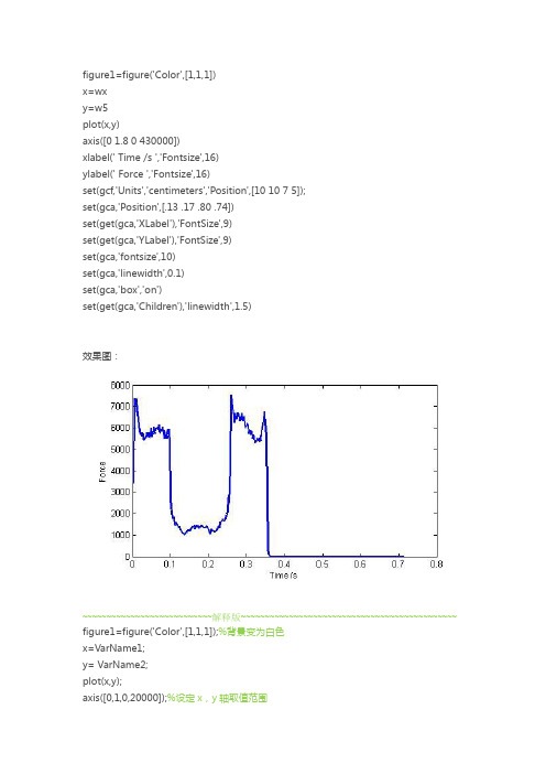
figure1=figure('Color',[1,1,1])x=wxy=w5plot(x,y)axis([01.80430000])xlabel('Time /s','Fontsize',16)ylabel('Force','Fontsize',16)set(gcf,'Units','centimeters','Position',[10 10 7 5]);set(gca,'Position',[.13 .17 .80 .74])set(get(gca,'XLabel'),'FontSize',9)set(get(gca,'YLabel'),'FontSize',9)set(gca,'fontsize',10)set(gca,'linewidth',0.1)set(gca,'box','on')set(get(gca,'Children'),'linewidth',1.5)效果图：~~~~~~~~~~~~~~~~~~~~~~~~~~~解释版~~~~~~~~~~~~~~~~~~~~~~~~~~~~~~~~~~~~~~~~~~~~~ figure1=figure('Color',[1,1,1]);%背景变为白色x=VarName1;y=VarName2;plot(x,y);axis([0,1,0,20000]);%设定x，y轴取值范围xlabel('Plastic stress','Fontsize',16);%X轴标签ylabel('Yeild stress /MPa','Fontsize',16);%Y轴标签%title(‘DP980应力应变曲线’,’Fontsize’,16);%标题%text(x,y, 'String');%在指定位置添加文本说明set(gcf,'Units','centimeters','Position',[10 10 7 5]);%设置图片大小为7cm×5cm%get hanlde to current axis返回当前图形的当前坐标轴的句柄,%(the first element is the relative distance of the axes to the left edge of the figure,... %the second the vertical distance from the bottom, and then the width and height; set(gca,'Position',[.13 .17 .80 .74]);%设置xy轴在图片中占的比例set(get(gca,'XLabel'),'FontSize',9);%图上文字为9 point或小5号set(get(gca,'YLabel'),'FontSize',9);%set(get(gca,'TITLE'),'FontSize',9);set(gca,'fontsize',9);set(gca,'linewidth',0.5); %坐标线粗0.5磅set(gca,'box','off');%Controls the box around the plotting areaset(get(gca,'Children'),'linewidth',1.5);%设置图中线宽1.5磅%set(gca,'color','r');%背景变为红色set(gcf,'Position',[100 100 260 220]);%这句是设置绘图的大小，不需要到word里再调整大小。

matlab方块排列代码方块排列是一种常见的图像处理和计算机视觉任务，它可以通过将图像分割为不同的方块，并按照一定规则重新排列来改变图像的外观。

在本文中，我们将探讨一些使用MATLAB编程语言实现方块排列的代码。

首先，我们需要加载一张图像作为输入。

我们可以使用MATLAB的imread函数来读取图像文件，该函数返回一个表示图像的矩阵。

例如，我们可以使用以下代码来加载名为"image.jpg"的图像：```image = imread('image.jpg');```接下来，我们需要确定方块的大小和形状。

一种常见的方法是将图像分割为正方形方块，但你也可以使用其他形状，如长方形或五边形。

在本文中，我们将使用正方形方块。

假设我们要将图像分割为NxN个方块，我们可以使用MATLAB的imresize函数来调整图像的大小，使得每个方块的大小为像素值为MxM。

以下是实现这一步骤的代码：```N = 10; % 每行/列的方块数量M = size(image, 1) / N; % 每个方块的像素数量resized_image = imresize(image, [M*N, M*N]);```接下来，我们需要创建一个空的画布来存储重新排列后的方块。

我们可以使用MATLAB的zeros函数创建一个MxMx3的矩阵，其中3表示每个像素的RGB值。

以下是实现这一步骤的代码：```canvas = zeros(M*N, M*N, 3);```现在，我们可以开始对图像进行方块排列。

我们可以使用两个嵌套的for循环来迭代遍历输入图像中的每个方块，并将其复制到我们创建的画布上的相应位置。

以下是实现这一步骤的代码：```for i = 1:Nfor j = 1:Nx = (i - 1) * M + 1;y = (j - 1) * M + 1;canvas(x:x+M-1, y:y+M-1, :) = resized_image((j-1)*M+1:j*M, (i-1)*M+1:i*M, :);endend```最后，我们可以使用MATLAB的imshow函数显示重新排列后的图像。

matlab画立体蝴蝶的代码Matlab是一款强大的工具，可以帮助我们完成许多数据分析、数学建模和图像处理等工作。

在Matlab中，我们可以用简单的代码绘制出许多精美的图像，例如立体蝴蝶。

下面就来介绍一下如何使用Matlab绘制立体蝴蝶的代码。

1.准备工作我们需要在Matlab中打开一个新的文件，然后输入下面这句代码创建一个3D画布：figure('units','normalized','outerposition',[0 0 1 1])这句代码将创建一个全屏的3D画布，供我们后续用来绘制立体蝴蝶。

2.绘制蝴蝶的翅膀接下来，我们需要定义蝴蝶的两个翅膀，具体代码如下：t = 0:pi/10:2*pi;x = sin(t).*(exp(cos(t))-2*cos(4*t)-sin(t/12).^5);y = cos(t).*(exp(cos(t))-2*cos(4*t)-sin(t/12).^5);z = sin(t/2).^2.*cos(5*t+pi/2);plot3(x,y,z,'r','LineWidth',2)这段代码的意思是先设置一个参数t，然后用该参数计算出x、y、z坐标分别对应蝴蝶翅膀上的点的位置。

最后使用plot3函数将这些点连接起来，形成一个立体的蝴蝶翅膀。

这时我们已经完成了蝴蝶的一只翅膀的绘制。

接下来我们需要将另一只翅膀按照一定的规律旋转、平移后绘制出来。

代码如下：hold onfor i=1:3xx = x*cos(pi*i/3) + y*sin(pi*i/3) - 5*(cos(pi*i/3)+1)/2; yy = -x*sin(pi*i/3) + y*cos(pi*i/3);zz = z+2*i;plot3(xx,yy,zz,'r','LineWidth',2)end这段代码首先使用for循环来遍历翅膀的三个位置。

%% 视觉错觉图-%% copyright&copy; 2007-2011 $author: baby_wolf $% $25-Dec-2011 00:25:14$%%clear allclose allhfig=figure('menu','none','pos',[200 200 800 300],'color','k') ; hold onaxis([0 1 -2 2]);axis off%% 标注text(0.01,1.1,'赵鸿平','color',[0.5 0.06 0.9],'fontsize',8);%% 点图t=0:1/480:479/480;y=sin(30*2*pi*t).*sin(2*pi*t);hplot=plot(t,y,'g.','markersize',3);%% 设置 gif 图片帧数等numFrames=30;frames = struct('cdata', [], 'colormap', []);frames(numFrames) = frames;%% 循环绘制各帧k=0;while k<=30%ishandle(hfig)y=y([17:end,1:16]);set(hplot,'xdata',t,'ydata',y); %点图移动pause(0.1);k=k+1;frames(k)=getframe(gcf); %获取当前帧end%% 写gif文件animated(1,1,1,numFrames) = 0;for k=1:numFramesif k == 1[animated, cmap] = rgb2ind(frames(k).cdata, 256, 'nodither');elseanimated(:,:,1,k) =rgb2ind(frames(k).cdata, cmap, 'nodither'); endend%%filename = 'illusorygif2.gif';if ~exist(filename,'file');imwrite(animated, cmap, filename, 'DelayTime', 0.1,'LoopCount', inf); endweb(filename)%%%close allclear all%% 设置N=520; %设置图像宽度Lwidth=12; %设置方块间隔宽度Swidth=60; %设置方块宽度Pwidth=Lwidth+Swidth;I=ones(N,N)*0.5;% I(:,:,1)=0;% I(:,:,2)=0.8;% I(:,:,3)=1;for i=Lwidth:Pwidth:N-Pwidth for j=Lwidth:Pwidth:N-PwidthI(i:i+Swidth-1,j:j+Swidth-1)=0;% I(i:i+29,j:j+29,2)=0;% I(i:i+29,j:j+29,3)=0;endendimshow(I);hold onfor i=(Pwidth+Lwidth/2):Pwidth:N-Pwidthfor j=(Pwidth+Lwidth/2):Pwidth:N-Pwidth%plot(i,j,'o','markersize',0.8*Lwidth,'markerfacecolor','w','markeredgec olor','none');endendcolormap hot%by baby_wolf%2011-12-23clear all;block_size=24;I1=[ones(block_size,block_size),zeros(block_size,block_size)]; I1=repmat(I1,1,6);I=repmat(I1,12,1);TMP=I1;for i=2:12% if rem(i,2)==1% n=-12;% else% n=8;% endn=randsample([-12 -8 6 10],1);if n>0TMP=TMP(:,[end-n:end 1:end-n-1]);elseTMP=TMP(:,[-n+1:end 1:-n]);endind=(i-1)*block_size+1;I(ind:ind+block_size-1,:)=TMP;endI(block_size:block_size:end,:)=0.3;imshow(I)colormap summer。