(英文)量子力学-薛定谔方程
- 格式:ppt
- 大小:717.00 KB
- 文档页数:30
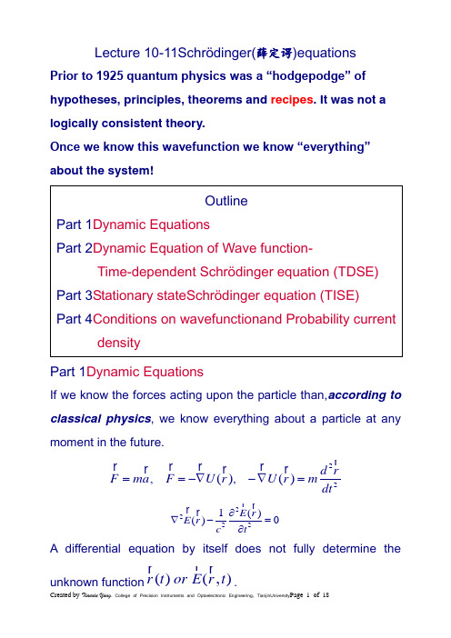
Lecture 10-11Schrödinger(薛定谔)equationsPrior to 1925 quantum physics was a “hodgepodge” of hypotheses, principles, theorems and recipes . It was not a logically consistent theory.Once we know this wavefunction we know “everything” about the system!Part 1Dynamic EquationsIf we know the forces acting upon the particle than,according to classical physics , we know everything about a particle at any moment in the future.22,(),()d r F ma F U r U r m dt ==-∇-∇=r r r r r r r r22221()()0E r E r c t∂∇-=∂r r r r A differential equation by itself does not fully determine theunknown function ()(,)r t or E r t r r r .Part 2Dynamic Equation of Wave function---- Schrödinger equations用21()sin cos 2x kx kx ψ⎡⎤=+⎢⎥⎣⎦描述的粒子,只能有5种动量取值,分别是0,2,2,,k k k k -- ,对应的几率分别是11111,,,,28888,这些几率总和应该为1。
()()1111111()0220,2888811111()128888ki i i k i i p P p p k k k k P p ====⋅+⋅+-⋅+⋅+-⋅==++++=∑∑h h h h 1212(),()1(),()1(),()1k ki i i i i x P x x P x x p x xd x x p x dx x x xd x x d ψψ=======⇒=∑∑⎰⎰⎰⎰¡¡¡¡Do we have the same recipe for calculation of average momentum by using wave function in position representation? Yes, of course, we have!To find the expectation (average) value of p , we first need to represent p in terms of x and t . Consider the derivative of the wave function of a free particle with respect to x:0001(,)exp ()p i x t p x E t ⎡⎤ψ=-⎢⎥⎣⎦h We find that0000000000**000(,)(,)(,)(,)(,)()(,)(,)(,)(0)δ∂ψ=ψ⇒ψ=ψ∂∂==ψ-ψ=ψψ=∂∂-∂⎰⎰p p p p p p p p i x t p x t x t p x t x p p x t i x t dx p x t x t dx i xp x h h h This suggests we define the momentum operator asThe expectation value of the momentum is20022220221()sin cos 2()()()()()=()()()()()ψϕϕϕϕϕ------⎡⎤=+⎢⎥⎣⎦=--++--++k k k k k k k k k k k k x kx kx C x C x C x C x C x x x x x x h h h h h h h h h h h h1()px i p x e ϕ=h ()()111111()022028888===⋅+⋅+-⋅+⋅+-⋅=∑ki i i p P p p k k k k h h h h So,we can not have definite values for the dynamical variables, such as the momentum, when the state of a particle is determined by the wave function with respect to x. We have to find the other way to describe thedynamical variables in Quantum Mechanics.For every dynamical variable or any observable thereis a corresponding Quantum Mechanical OperatorPhysical Quantities →OperatorsOperators are important in quantum mechanics. All observables have corresponding operators.Operators ↔Symbols for mathematical operation✧ The position x is its own operator ˆxx =. Done. Other operators are simpler and just involve multiplication 22x x x x ∧==⋅. ✧ The potential energy operator is just multiplication by V(x).✧ The momentum operator is defined as ˆp i x ∂=-∂h00000002211ˆˆˆˆ1()()[11ˆ(()](())()222ˆ()()())ˆ()()1ˆ()2pp xipp x p xp xix x piix px p pp xix p pp p ppx eipip x i e p eexp x p xx xpT x p p x p p x xpxx eT x T xϕϕϕϕμμμϕϕϕϕϕϕϕμϕ=====⎛⎫∂-=-==⎪∂⎝⎭===hh hhhhh()px xϕ=h000000001(,)exp()1ˆ(,)exp()(,)ˆ(,)(,)pp pp pix t p x E ti iEE x t i p x E t i x ttE x t E x t⎡⎤ψ=-⎢⎥⎣⎦∂⎧⎫⎡⎤⎛⎫ψ=-=ψ-⎬ ⎪⎢⎥∂⎝⎭⎣⎦⎭ψ=ψhh hh h Eigenvalue equation of an operatoreigenvalueDeriving the Schrödinger Equation using operators: This was a plausibility argument, not a derivation. We believe the Schrödinger equation not because of this argument, but because its predictions agree withexperiments.Schrödinger EquationNotes:The Schrödinger Equation is THE fundamental equation of Quantum Mechanics.There are limits to its validity. In this form it applies only to a single, non-relativistic particle (i.e. one withnon-zero rest mass and speed much less than c.)●On the left hand picture 13 velocity vectors of an individual fly are shown; the chain●On the right hand picture the same 13velocity vectors are assigned to 1 fly each todemonstrate that the ensemble average yields the same result, i.e. <v e> = 0,provided that each and every fly does the same thing on average.●i.e. time average = ensemble average. The new subscripts "e" and "r" denote ensemble and space, respectively. This is a simple version of a very far reaching concept in stochastic physics known under the catch word "ergodic hypothesis".●As long as every fly does - on average - the same thing, the vector average overtime of the ensemble is identical to that of an individual fly - if we sum up a fewthousand vectors for one fly, or a few million for lots of flies does not make anydifference. However, we also may obtain this average in a different way:●We do not average one fly in time obtaining <v i>t , but at any given time all flies inspace.●This means, we just add up the velocity vectors of all flies at some moment in timeand obtain <v e>r , the ensemble average. It is evident (but not easy to prove for general cases) thata) Schrödinger equation is a linear homogeneous partialdifferential equation.b) The Schrödinger equation contains the complex number i.Therefore its solutions are essentially complex (unlikeclassical waves, where the use of complex numbers isjust a mathematical convenience.)c) The wave equation has infinite number of solutions,someof which do not correspond to any physical or chemical reality.1. For an electron bound to an atom/molecule, the wavefunction must be everywhere finite, and it must vanish in the boundaries2. Single valued3. Continuous4. Gradient (dψ/dr) must be continuous5. ψψ*dτ is finite, so that ψ can be normalizedd) Solutions that do not satisfy these properties(above)DONOT generally correspond to physicallyrealizable circumstances.e) Conditions on the wave function(波函数的三个基本条件——有限、单值、连续)1. In order to avoid infinite probabilities, the wave functionmust be finite everywhere.2. The wave function must be single valued.3. The wave function must be twice differentiable. Thismeans that it and its derivative must be continuous. (An exception to this rule occurs when V is infinite.)4. In order to normalize a wave function, it must approachzero as x approaches infinity.f) Only the physically measurable quantities must be real.These include the probability, momentum and energy.Can think of the LHS of the Schrödinger equation as a differentialoperator that represents the energy of the particle ?This operator is called the Hamiltonian of the particle , and usually given the symbolˆH.Hamiltonian is a linear differential operator .222ˆ(,)2d V x t H m dx ⎡⎤-+ψ≡ψ⎢⎥⎣⎦h Kineticenergy Potential energyHence there is an alternative (shorthand) form for thetime-dependent Schrödinger equation:Part 3Time-independent Schrödinger equation (TISE), i.e.stationary state(定态)Schrödinger equationSuppose potential is independent of time(),()U x t U x =Look for a separated solution, substitute (,)()()x t x T t ψψ=into• This only tells us that T(t) depends on the energy E . It doesn’t tell us what the energy actually is. For that we have to solve the space part.• T(t) does not depend explicitly on the potential U(x). But there is an implicit dependencebecause the potential affectsthe possible values for the energy E .This is the time-independent Schrödinger equation (TISE) or so-called stationary state Schrödinger equation.Solution to full TDSE isEven though the potential is independent of time the wavefunction still oscillates in time . But probability distribution is static()()2*//2*,,()()()()()iEt iEt P x t x t x e x e x x x ψψψψψ+-=ψ===h hFor this reason a solution of the TISE is known as a StationaryState(定态)Stationary state Schrödinger Equation Notes:• In one-dimension space, the TISE is an ordinary differential equation (not a partial differential equation)• The TISE is an eigenvalue equation for the Hamiltonianoperator:ˆ()()Hx E x ψψ=Part 4 Probability current density and continuity equation Definition of probability current densityIn non-relativistic quantum mechanics, the probability current of the wave function Ψ is defined asin the position basis and satisfies the quantum mechanical continuity equationwith the probability density defined as.If one were to integrate both sides of the continuity equation with respect to volume, so thatthen the divergence theorem implies the continuity equation is equivalent to the integral equationwhere the V is any volume and S is the boundary of V. This is the conservation law for probability in quantum mechanics.In particular, if is a wavefunction describing a single particle, theintegral in the first term of the preceding equation (without the time derivative) is the probability of obtaining a value within V when the position of the particle is measured. The second term is then the rate at which probability is flowing out of the volume V. Altogether the equation states that the time derivative of the change of the probability of the particle being measured in V is equal to the rate at which probability flows into V. Derivation of continuity equationThe continuity equation is derived from the definition of probability current and the basic principles of quantum mechanics. Suppose is the wavefunction for a single particle in the positionbasis (i.e. is a function of x, y, and z). Thenis the probability that a measurement of the particle's position will yield a value within V. The time derivative of this iswhere the last equality follows from the product rule and the fact that the shape of V is presumed to be independent of time (i.e. the time derivative can be moved through the integral). In order to simplify this further, consider the time dependent Schrödinger equationand use it to solve for the time derivative of :When substituted back into the preceding equation for this gives.Now from the product rule for the divergence operatorand since the first and third terms cancel:If we now recall the expression for P and note that the argumentof the divergence operator is justthis becomeswhich is the integral form of the continuity equation .The differential form follows from the fact that the preceding equation holds for all V, and as the integrand is a continuousfunction of space, it must vanish everywhere:For all whole space we have()()2lim lim 0lim lim 0V V V V V S V S dV j dV t j dV j ds →∞→∞→→∞→∞⎛⎫∂ψ ⎪=-∇⋅= ⎪∂⎝⎭∇⋅=⋅=⎰⎰⎰⎰⎰⎰⎰⎰⎰⎰⎰r r r r rwhich meansthat must be continuousat any positionin the whole space.So the wavefunction and its derivative must be continuous.(An exception to this rule occurs when V is infinite.)One more, if the(,)()Et i x t x e ϕ-ψ=hand ()x ϕis real, the probability current*Im ()()0j x x m ϕϕ⎡⎤=∇≡⎣⎦r r h over the whole 1D space which means j r is always continuous whatever the wavefunction ()x ϕand its derivative ()x ϕ'are continuous or not. However, ()x ϕhas to be continuous for an acceptable physical solution for that the probability density is uniquely defined(唯一确定). As to ()x ϕ', it may not be continuous especially at the point where the potential energy is infinite.It is easy to prove that ()x ϕ' has to be continuous at the point 0x where the potential energy just has a limited high step.Have a fun!。

薛定谔方程(英语:Schrodinger equation)是由奥地利物理学家薛定谔在1926年提出的一个用于描述量子力学中波函数的运动方程[1],被认为是量子力学的奠基理论之一。
薛定谔方程主要分为含时薛定谔方程与不含时薛定谔方程。
含时薛定谔方程相依于时间,专门用来计算一个量子系统的波函数,怎样随着时间演变。
不含时薛定谔方程不相依于时间,可以计算一个定态量子系统,对应于某本征能量的本征波函数。
波函数又可以用来计算,在量子系统里,某个事件发生的概率幅。
而概率幅的绝对值的平方,就是事件发生的概率密度。
薛定谔方程的解答,清楚地描述量子系统里,量子尺寸粒子的统计性量子行为。
量子尺寸的粒子包括基本粒子,像电子、质子、正电子、等等,与一组相同或不相同的粒子,像原子核。
薛定谔方程可以转换为海森堡的矩阵力学,或费曼的路径积分表述 (path integral formulation) 。
薛定谔方程是个非相对论性的方程,不能够用于相对论性理论。
海森堡表述比较没有这么严重的问题;而费曼的路径积分表述则完全没有这方面的问题。
[编辑]含时薛定谔方程虽然,含时薛定谔方程能够启发式地从几个假设导引出来。
理论上,我们可以直接地将这方程当作一个基本假定。
在一维空间里,一个单独粒子运动于位势中的含时薛定谔方程为(1)其中,是质量,是位置,是相依于时间的波函数,是约化普朗克常数,是位势。
类似地,在三维空间里,一个单独粒子运动于位势中的含时薛定谔方程为(2)假若,系统内有个粒子,则波函数是定义于-位形空间,所有可能的粒子位置空间。
用方程表达,。
其中,波函数的第个参数是第个粒子的位置。
所以,第个粒子的位置是。
[编辑]不含时薛定谔方程不含时薛定谔方程不相依于时间,又称为本征能量薛定谔方程,或定态薛定谔方程。
顾名思义,本征能量薛定谔方程,可以用来计算粒子的本征能量与其它相关的量子性质。
应用分离变量法,猜想的函数形式为;其中,是分离常数,是对应于的函数.稍回儿,我们会察觉就是能量.代入这猜想解,经过一番运算,含时薛定谔方程 (1) 会变为不含时薛定谔方程:。

爱因斯坦薛定谔方程
爱因斯坦-薛定谔方程(Einstein-Schrödinger equation)是一个量子力学中的方程,将爱因斯坦的相对论和薛定谔方程结合在一起,描述了物质和场相互作用的行为。
这个方程是在广义相对论和量子力学之间的理论框架下提出的。
具体而言,爱因斯坦-薛定谔方程描述了物质在引力场中的行为,以及粒子与电磁场的相互作用。
它是一个偏微分方程,通常被写成:iħ∂ψ/∂t = (c^2√(p^2c^2 + m^2c^4) + eφ)ψ。
其中,ψ是波函数,描述了量子态的演化;t是时间;ħ是约化普朗克常数;c是光速;p是动量算符;m是粒子的静质量;e是元电荷;φ是电磁场势。
爱因斯坦-薛定谔方程是一个非常复杂的方程,它描述了物质在引力场和电磁场中的量子行为。
这个方程在理论物理的研究中扮演着重要的角色,帮助我们理解微观世界的行为。
但是,由于其复杂性,解析解很难找到,通常需要使用数值方法进行求解。


七个薛定谔方程薛定谔方程是量子力学中描述粒子行为的基本方程。
一般情况下,薛定谔方程可以写成如下的形式:1. 定态薛定谔方程(Stationary Schrödinger Equation):iħ∂Ψ/∂t = HΨ其中,ħ是约化普朗克常数,Ψ是波函数,t是时间,H是哈密顿算符。
2. 非定态薛定谔方程(Time-dependent Schrödinger Equation):iħ∂Ψ/∂t = HΨ其中,Ψ是波函数,t是时间,H是哈密顿算符。
3. 薛定谔方程的波函数形式(Schrödinger Equation in Wave Function Form):iħ∂Ψ/∂t = -ħ²/2m ∇²Ψ + VΨ其中,ħ是约化普朗克常数,m是粒子质量,Ψ是波函数,t是时间,∇²是拉普拉斯算符,V是势能函数。
4. 薛定谔方程的路径积分形式(Path Integral Form of Schrödinger Equation):Ψ(x,t) = ∫ Dx exp(iS[x]/ħ)Ψ(x₀,0)其中,Ψ(x,t)是波函数,S[x]是作用量,x₀是初始位置,Dx是路径积分测度。
5. 一维薛定谔方程(One-Dimensional Schrödinger Equation):iħ∂Ψ/∂t = -ħ²/2m ∂²Ψ/∂x² + V(x)Ψ其中,ħ是约化普朗克常数,m是粒子质量,Ψ是波函数,t是时间,x是位置,V(x)是势能函数。
6. 三维薛定谔方程(Three-Dimensional Schrödinger Equation):iħ∂Ψ/∂t = -ħ²/2m ∇²Ψ + V(r)Ψ其中,ħ是约化普朗克常数,m是粒子质量,Ψ是波函数,t是时间,r是位置矢量,∇²是拉普拉斯算符,V(r)是势能函数。

量子力学英语
量子力学是一种描述微观世界的理论,在实验中已被证明具有极高的准确性。
虽然量子力学的概念和数学语言非常抽象,但它已成为许多现代科技和工程领域的基础。
因此,对于学习和研究量子力学的人来说,掌握一些相关的英语词汇和表达方式是非常重要的。
以下是一些量子力学英语词汇和表达方式的例子:
1. Quantum mechanics - 量子力学
2. Wave function - 波函数
3. Superposition principle - 叠加原理
4. Uncertainty principle - 不确定性原理
5. Entanglement - 纠缠态
6. Quantum state - 量子态
7. Measurement - 测量
8. Eigenstate - 本征态
9. Operator - 算符
10. Hamiltonian - 哈密顿量
11. Schrdinger equation - 薛定谔方程
12. Commutation - 对易关系
13. Hermitian operator - 厄米算符
14. Unitary operator - 酉算符
15. Quantum field theory - 量子场论
通过学习这些量子力学英语词汇和表达方式,可以更好地理解和
交流量子力学相关的概念和研究成果。
薛定谔方程(Schrodinger equation)是由奥地利物理学家薛定谔提出的量子力学中的一个基本方程,也是量子力学的一个基本假定,其正确性只能靠实验来检验。
它是将物质波的概念和波动方程相结合建立的二阶偏微分方程,可描述微观粒子的运动,每个微观系统都有一个相应的薛定谔方程式,通过解方程可得到波函数的具体形式以及对应的能量,从而了解微观系统的性质。
1定义薛定谔方程薛定谔方程(Schrodinger equation)又称薛定谔波动方程(Schrodinger wave equation)在量子力学中,体系的状态不能用力学量(例如x)的值来确定,而是要用力学量的函数Ψ(x,t),即波函数(又称概率幅,态函数)来确定,因此波函数成为量子力学研究的主要对象。
力学量取值的概率分布如何,这个分布随时间如何变化,这些问题都可以通过求解波函数的薛定谔方程得到解答。
这个方程是奥地利物理学家薛定谔于1926年提出的,它是量子力学最基本的方程之一,在量子力学中的地位与牛顿方程在经典力学中的地位相当。
薛定谔方程是量子力学最基本的方程,亦是量子力学的一个基本假定,其正确性只能靠实验来确定。
2方程概述量子力学中求解粒子问题常归结为解薛定谔方程或定态薛定谔方程。
薛定谔方程广泛地用于原子物理、核物理和固体物理,对于原子、分子、核、固体等一系列问题中求解的结果都与实际符合得很好。
薛定谔方程仅适用于速度不太大的非相对论粒子,其中也没有包含关于粒子自旋的描述。
当涉及相对论效应时,薛定谔方程由相对论量子力学方程所取代,其中自然包含了粒子的自旋。
.薛定谔提出的量子力学基本方程。
建立于1926年。
它是一个非相对论的波动方程。
它反映了描述微观粒子的状态随时间变化的规律,它在量子力学中的地位相当于牛顿定律对于经典力学一样,是量子力学的基本假设之一。
设描述微观粒子状态的波函数为Ψ(r,t),质量为m的微观粒子在势场V(r,t)中运动的薛定谔方程为。
1、microscopic world 微观世界2、macroscopic world 宏观世界3、quantum theory 量子[理]论4、quantum mechanics 量子力学5、wave mechanics 波动力学6、matrix mechanics 矩阵力学7、Planck constant 普朗克常数8、wave-particle duality 波粒二象性9、state 态10、state function 态函数11、state vector 态矢量12、superposition principle of state 态叠加原理13、orthogonal states 正交态14、antisymmetrical state 正交定理15、stationary state 对称态16、antisymmetrical state 反对称态17、stationary state 定态18、ground state 基态19、excited state 受激态20、binding state 束缚态21、unbound state 非束缚态22、degenerate state 简并态23、degenerate system 简并系24、non-deenerate state 非简并态25、non-degenerate system 非简并系26、de Broglie wave 德布罗意波27、wave function 波函数28、time-dependent wave function 含时波函数29、wave packet 波包30、probability 几率31、probability amplitude 几率幅32、probability density 几率密度33、quantum ensemble 量子系综34、wave equation 波动方程35、Schrodinger equation 薛定谔方程36、Potential well 势阱37、Potential barrien 势垒38、potential barrier penetration 势垒贯穿39、tunnel effect 隧道效应40、linear harmonic oscillator线性谐振子41、zero proint energy 零点能42、central field 辏力场43、Coulomb field 库仑场44、δ-function δ-函数45、operator 算符46、commuting operators 对易算符47、anticommuting operators 反对易算符48、complex conjugate operator 复共轭算符49、Hermitian conjugate operator 厄米共轭算符50、Hermitian operator 厄米算符51、momentum operator 动量算符52、energy operator 能量算符53、Hamiltonian operator 哈密顿算符54、angular momentum operator 角动量算符55、spin operator 自旋算符56、eigen value 本征值57、secular equation 久期方程58、observable 可观察量59、orthogonality 正交性60、completeness 完全性61、closure property 封闭性62、normalization 归一化63、orthonormalized functions 正交归一化函数64、quantum number 量子数65、principal quantum number 主量子数66、radial quantum number 径向量子数67、angular quantum number 角量子数68、magnetic quantum number 磁量子数69、uncertainty relation 测不准关系70、principle of complementarity 并协原理71、quantum Poisson bracket 量子泊松括号72、representation 表象73、coordinate representation 坐标表象74、momentum representation 动量表象75、energy representation 能量表象76、Schrodinger representation 薛定谔表象77、Heisenberg representation 海森伯表象78、interaction representation 相互作用表象79、occupation number representation 粒子数表象80、Dirac symbol 狄拉克符号81、ket vector 右矢量82、bra vector 左矢量83、basis vector 基矢量84、basis ket 基右矢85、basis bra 基左矢86、orthogonal kets 正交右矢87、orthogonal bras 正交左矢88、symmetrical kets 对称右矢89、antisymmetrical kets 反对称右矢90、Hilbert space 希耳伯空间91、perturbation theory 微扰理论92、stationary perturbation theory 定态微扰论93、time-dependent perturbation theory 含时微扰论94、Wentzel-Kramers-Brillouin method W. K. B.近似法95、elastic scattering 弹性散射96、inelastic scattering 非弹性散射97、scattering cross-section 散射截面98、partial wave method 分波法99、Born approximation 玻恩近似法100、centre-of-mass coordinates 质心坐标系101、laboratory coordinates 实验室坐标系102、transition 跃迁103、dipole transition 偶极子跃迁104、selection rule 选择定则105、spin 自旋106、electron spin 电子自旋107、spin quantum number 自旋量子数108、spin wave function 自旋波函数109、coupling 耦合110、vector-coupling coefficient 矢量耦合系数111、many-partic le system 多子体系112、exchange forece 交换力113、exchange energy 交换能114、Heitler-London approximation 海特勒-伦敦近似法115、Hartree-Fock equation 哈特里-福克方程116、self-consistent field 自洽场117、Thomas-Fermi equation 托马斯-费米方程118、second quantization 二次量子化119、identical particles全同粒子120、Pauli matrices 泡利矩阵121、Pauli equation 泡利方程122、Pauli’s exclusion principle泡利不相容原理123、Relativistic wave equation 相对论性波动方程124、Klein-Gordon equation 克莱因-戈登方程125、Dirac equation 狄拉克方程126、Dirac hole theory 狄拉克空穴理论127、negative energy state 负能态128、negative probability 负几率129、microscopic causality 微观因果性本征矢量eigenvector本征态eigenstate本征值eigenvalue本征值方程eigenvalue equation本征子空间eigensubspace (可以理解为本征矢空间)变分法variatinial method标量scalar算符operator表象representation表象变换transformation of representation表象理论theory of representation波函数wave function波恩近似Born approximation玻色子boson费米子fermion不确定关系uncertainty relation狄拉克方程Dirac equation狄拉克记号Dirac symbol定态stationary state定态微扰法time-independent perturbation定态薛定谔方程time-independent Schro(此处上面有两点)dinger equation 动量表象momentum representation角动量表象angular mommentum representation占有数表象occupation number representation坐标(位置)表象position representation角动量算符angular mommentum operator角动量耦合coupling of angular mommentum对称性symmetry对易关系commutator厄米算符hermitian operator厄米多项式Hermite polynomial分量component光的发射emission of light光的吸收absorption of light受激发射excited emission自发发射spontaneous emission轨道角动量orbital angular momentum自旋角动量spin angular momentum轨道磁矩orbital magnetic moment归一化normalization哈密顿hamiltonion黑体辐射black body radiation康普顿散射Compton scattering基矢basis vector基态ground state基右矢basis ket ‘右矢’ket基左矢basis bra简并度degenerancy精细结构fine structure径向方程radial equation久期方程secular equation量子化quantization矩阵matrix模module模方square of module内积inner product逆算符inverse operator欧拉角Eular angles泡利矩阵Pauli matrix平均值expectation value (期望值)泡利不相容原理Pauli exclusion principle氢原子hydrogen atom球鞋函数spherical harmonics全同粒子identical partic les塞曼效应Zeeman effect上升下降算符raising and lowering operator 消灭算符destruction operator产生算符creation operator矢量空间vector space守恒定律conservation law守恒量conservation quantity投影projection投影算符projection operator微扰法pertubation method希尔伯特空间Hilbert space线性算符linear operator线性无关linear independence谐振子harmonic oscillator选择定则selection rule幺正变换unitary transformation幺正算符unitary operator宇称parity跃迁transition运动方程equation of motion正交归一性orthonormalization正交性orthogonality转动rotation自旋磁矩spin magnetic monent(以上是量子力学中的主要英语词汇,有些未涉及到的可以自由组合。
薛定谔方程一般表达式
薛定谔方程是描述量子力学中粒子的运动和性质的方程。
一般表达式为:
Hψ = Eψ
其中,H是哈密顿算符,ψ是波函数,E是能量。
在一维情况下,薛定谔方程可以写成:
-ħ²/2m * ∂²ψ/∂x² + V(x)ψ = Eψ
其中,ħ是普朗克常数除以2π,m是粒子的质量,V(x)是势能函数,E是粒子的能量。
在三维情况下,薛定谔方程可以写成:
-ħ²/2m * (∂²ψ/∂x² + ∂²ψ/∂y² + ∂²ψ/∂z²) + V(x, y, z)ψ = Eψ
其中,x、y、z是空间坐标,V(x, y, z)是势能函数,E是粒子的能量。
这些方程描述了波函数随时间和空间的变化,通过求解薛定谔方程,可以得到粒子的波函数以及与波函数相关的物理量,如能量、位置、动量等。