机器人学导论第4章1
- 格式:ppt
- 大小:3.25 MB
- 文档页数:33
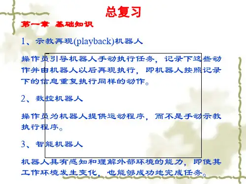
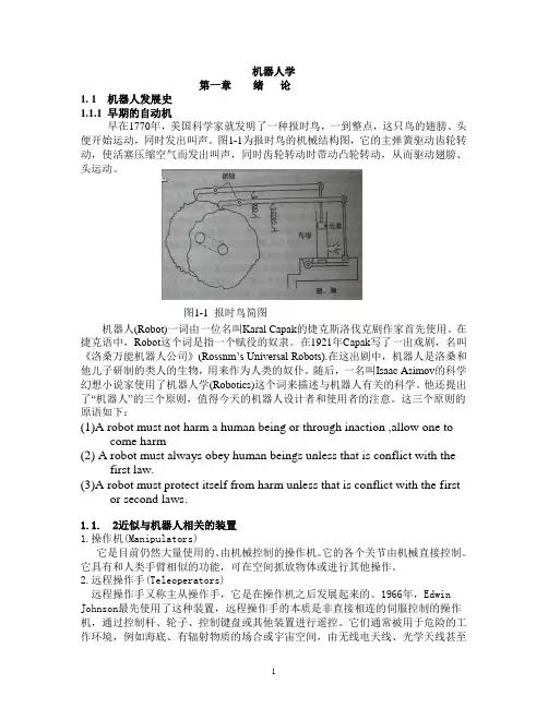
机器人学第一章绪论1. 1 机器人发展史1.1.1 早期的自动机早在1770年,美国科学家就发明了一种报时鸟,一到整点,这只鸟的翅膀、头便开始运动,同时发出叫声。
图1-1为报时鸟的机械结构图,它的主弹簧驱动齿轮转动,使活塞压缩空气而发出叫声,同时齿轮转动时带动凸轮转动,从而驱动翅膀、头运动。
图1-1 报时鸟简图机器人(Robot)一词由一位名叫Karal Capak的捷克斯洛伐克剧作家首先使用。
在捷克语中,Robot这个词是指一个赋役的奴隶。
在1921年Capak写了一出戏剧,名叫《洛桑万能机器人公司》(Rossnm’s Universal Robots).在这出剧中,机器人是洛桑和他儿子研制的类人的生物,用来作为人类的奴仆。
随后,一名叫Isaac Asimov的科学幻想小说家使用了机器人学(Robotics)这个词来描述与机器人有关的科学。
他还提出了“机器人”的三个原则,值得今天的机器人设计者和使用者的注意。
这三个原则的原语如下:(1)A robot must not harm a human being or through inaction ,allow one tocome harm(2) A robot must always obey human beings unless that is conflict with thefirst law.(3)A robot must protect itself from harm unless that is conflict with the firstor second laws.1.1.2近似与机器人相关的装置1.操作机(Manipulators)它是目前仍然大量使用的、由机械控制的操作机。
它的各个关节由机械直接控制。
它具有和人类手臂相似的功能,可在空间抓放物体或进行其他操作。
2.远程操作手(Teleoperators)远程操作手又称主从操作手,它是在操作机之后发展起来的。
机器人学导论第三章:机器人建模与表示3.1 机器人模型机器人模型是机器人学中最重要的概念之一。
它描述了机器人的物理特征和行为。
机器人模型可以是物理模型,也可以是数学模型。
3.1.1 物理模型物理模型是指将实际的机器人物理特征通过物体的尺寸、质量、结构等进行描述的模型。
物理模型可以用来研究机器人的运动、力学特性以及与环境的交互。
在物理模型中,常用的描述方法有刚体模型和柔软体模型。
刚体模型认为机器人的构件是刚性的,不会发生变形,而柔软体模型则考虑了机器人构件的弹性特性。
3.1.2 数学模型数学模型是指通过数学方程或函数来描述机器人的特征和行为的模型。
数学模型可以用来研究机器人的控制算法、运动规划、感知等问题。
常用的数学模型有几何模型、运动学模型、动力学模型等。
几何模型描述机器人的几何特征,如位置、姿态等;运动学模型描述机器人的运动学特性,如速度、加速度等;动力学模型描述机器人的力学特性,如力、力矩等。
3.2 机器人表示机器人表示是指将机器人的信息进行编码和存储的方法。
机器人表示可以是离散的或连续的,可以是静态的或动态的。
机器人的状态表示是对机器人在某一时刻的特征和行为进行编码的方法。
常用的状态表示方法有位姿表示、关节状态表示、力传感器状态表示等。
位姿表示是指用位置和方向来描述机器人的姿态。
常用的位姿表示方法有笛卡尔坐标表示和欧拉角表示。
关节状态表示是指用关节角度或关节位置来描述机器人的关节状态。
力传感器状态表示是指用力和力矩来描述机器人的外部力和力矩。
机器人的环境表示是对机器人周围环境的信息进行编码的方法。
常用的环境表示方法有场景图表示、网格地图表示、障碍物表示等。
场景图表示是指用图的形式表示机器人周围的物体及其关系。
网格地图表示是指将机器人周围的环境划分为一个个网格,每个网格表示一种状态。
障碍物表示是指用几何体或网格来表示机器人周围的障碍物。
3.3 机器人建模与表示的应用机器人建模与表示在机器人学中具有广泛的应用。
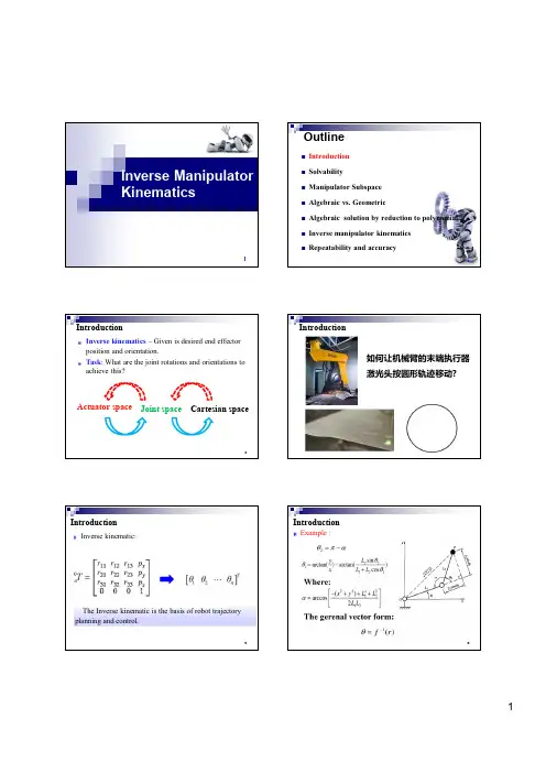
Inverse ManipulatorKinematicsAlgebraic solution by reduction to polynomialOutline2 Introduction IntroductionIntroductionThe Inverse kinematic is the basis of robot trajectory planning and control.5IntroductionExample :6Algebraic solution by reduction to polynomialOutline7SolvabilitySolvabilityFor the 6 DOF Puma 560 manipulator,we have:How to find the 6 joint variablesHere we might have 12 equations to solve for 6 independent variables. Constraints should be utilized.6 equations for 6 unknown variables9SolvabilityDifficulty: these 6 equations are nonlinear and transcendental equations.obtain the solution.whereSolvability11SolvabilitySolvabilityThe dexterous workspace is only one point(the origin). The There is no dexterous workspace. The reachable SolvabilityFor most industry robots, there is limitation for the joint variable range, thus the workspace is reduced.Only one attainable orientationIf a manipulator has less than 6 DOF, it can’t attain general goal position and orientation in 3D space.Workspace also depends on the tool-frame transformation.Solvability15There might be multiple solution in solving kinematic equations.Two possible solution for the same position and orientation.How to choose possible solution?Solvability” solution.The number of solutions depends on the number of and the allowable ranges of motion of the joints, also, it can be a function of other link parameters (link length, link twist, link offset, joint angle).Solvability2. Multiple solutions17The PUMA 560 can reach certain goals with 8different solutions.+Due to the limits of joints range, some of these 8 solutions could be inaccessible.SolvabilitySolvabilityAlgebraic solution by reduction to polynomial Outline20Manipulator Subspace21workspace is a portion of an n‐DOF subspacesubspace : planeworkspace : a subset of the plane{workspace} ⊂{subspace} ⊂{space}Manipulator Subspaceof a manipulator?Giving an expression for a manipulator’s wrist frame {w}to be free to take on all possible values.Manipulator SubspaceThe subspace of is given by:233R planar manipulatorAs are allowed to take on arbitrary values, the subspace is generatedNOTE : Link lengths and joints limits restrict the workspace of the manipulator to be a subset of this subspace.Algebraic solution by reduction to polynomial Outline24Algebraic vs. GeometricGiven the transformation matrix, solved for25Algebraic vs. GeometricD-H TableAlgebraic vs. GeometricThe transformation matrix can be computed viaand we haveAlgebraic vs. GeometricSpecification of the goal points can be accomplished by specifying three parameters: ..The transformation is assumed to have the following structurewhereThe above four nonlinear equations are used to solve for (unknown)Algebraic vs. GeometricThe parameters is How to solve for according thefollowing equations:Algebraic vs. Geometric1.Algebraic solution 30The is the only unknown parameter.Algebraic vs. GeometricStep1.In the solution algorithm, the above constraintshould be checked to determine whether a solution exist or not. If the constrain is not Algebraic vs. Geometric1.Algebraic solution Here, the choice of signs in the solution of corresponds to Algebraic vs. Geometric33Based on the solution of , we can get:whereAlgebraic vs. Geometricwe haveAlgebraic vs. GeometricNote:If a choice of sign is made in the solution of ,it will affect and thus affectStep5. Based on the fact that The solution of can be obtained.Algebraic vs. Geometric36solved for by using the tools of plane geometry.can utilize plane geometry directly to find a solution.Algebraic vs. Geometricconsidering the solid triangle, the “” can be applied to solve for as:37PossibleconfigurationThe other possible solution can be obtained by settingAlgebraic vs. Geometric2. Geometric solutionTo solve for , we find the express for angleand .38and can be solved via:then can be solved as:Algebraic vs. Geometric39the solution of can Algebraic solution by reduction to polynomial Outline40Algebraic solution by reduction to polynomialexpression in terms of a single variable.This is a very important geometric substitution used often in solving kinematic equations. These substitution convert transcendental equations into polynomial equations in Algebraic solution by reduction to polynomialGiven a transcendental equation try to solve for42Solutions:(when )Algebraic solution by reduction to polynomial Outline43Inverse manipulator kinematicsThe Unimation Puma 560 Industry Robot44Inverse manipulator kinematicsReview : D-H table45Inverse manipulator kinematicsReview : Transformation of each link.46Inverse manipulator kinematicsReview : Transformation of all link47whereInverse manipulator kinematics: Given the goal point and orientation specified by:(Known: Numerical value)Solve forInverse manipulator kinematics Separating out 1 unknown parameter How to solve ?Inverse manipulator kinematics2. Inverting to be obtain50 whereInverse manipulator kinematicsCheck the (2,4) elements on both sides ,we have Inverse manipulator kinematicsIntroduce the trigonometric(三角恒等变换) substitutions:52whereThen it can be obtained that:Inverse manipulator kinematics3. The left side of the following equation is known53Inverse manipulator kinematicsTaking square of the above two equations, and adding the results together, it can be obtained thatInverse manipulator kinematicsThe above equation depends only on , then similar steps can be followed to solve for as:4. Consider the following equationhave been solved, but is unknownInverse manipulator kinematics56Eq.(3.11) in Chapter3Check elements (1,4) and (2,4) on both sides, we haveInverse manipulator kinematics 57Inverse manipulator kinematics585. Now the left side of the following equation is knownEq.(3.11) in Chapter3Check the elements (1,3) and (3,3), it can be obtained thatInverse manipulator kinematics ca can be solved as:Case2.,The manipulator is in a singular configurationas axis 4 and 6 line up and cause the same motion of the last link of the robot. Thus is chosen arbitrarily.Inverse manipulator kinematics606. Consider the following equation again:andCheck the elements (1,3) and (3,3), it can be obtained thatInverse manipulator kinematics 61Hence, we can solve for as7. Applying the same method one more time, we havewhereCheck the elements (3,1) and (1,1), it can be obtained thatInverse manipulator kinematics62Thus we can solve for aswe can obtain eight sets of possible solutions, some of them will be discarded due to the joint angle limitsInverse manipulator kinematics63Summary1、原则:等号两端的矩阵中对应元素相等,列出相关方)、从含变量少的左边开始,如,向右递推,直到)、选择等号左边或右边矩阵中等于常数或仅含有一个变量的元素,列出相应元素对应的方程或方程组。


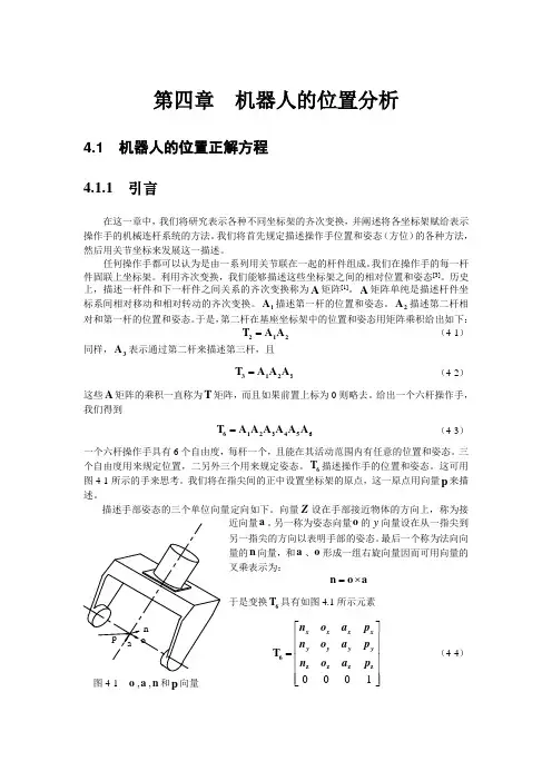
第四章 机器人的位置分析4.1 机器人的位置正解方程 4.1.1 引言在这一章中,我们将研究表示各种不同坐标架的齐次变换,并阐述将各坐标架赋给表示操作手的机械连杆系统的方法。
我们将首先规定描述操作手位置和姿态(方位)的各种方法,然后用关节坐标来发展这一描述。
任何操作手都可以认为是由一系列用关节联在一起的杆件组成。
我们在操作手的每一杆件固联上坐标架。
利用齐次变换,我们能够描述这些坐标架之间的相对位置和姿态[3]。
历史上,描述一杆件和下一杆件之间关系的齐次变换称为A 矩阵[1]。
A 矩阵单纯是描述杆件坐标系间相对移动和相对转动的齐次变换。
1A 描述第一杆的位置和姿态。
2A 描述第二杆相对和第一杆的位置和姿态。
于是,第二杆在基座坐标架中的位置和姿态用矩阵乘积给出如下:=212T A A (4-1) 同样,3A 表示通过第二杆来描述第三杆,且3=312T A A A (4-2)这些A 矩阵的乘积一直称为T 矩阵,而且如果前置上标为0则略去。
给出一个六杆操作手,我们得到36=61245T A A A A A A (4-3)一个六杆操作手具有6个自由度,每杆一个,且能在其活动范围内有任意的位置和姿态。
三个自由度用来规定位置,二另外三个用来规定姿态。
6T 描述操作手的位置和姿态。
这可用图4-1所示的手来思考。
我们将在指尖间的正中设置坐标架的原点,这一原点用向量p 来描述。
描述手部姿态的三个单位向量定向如下。
向量Z 设在手部接近物体的方向上,称为接近向量a 。
另一称为姿态向量o 的y 向量设在从一指尖到另一指尖的方向以表明手部的姿态。
最后一个称为法向向量的n 向量,和a 、o 形成一组右旋向量因而可用向量的叉乘表示为:=⨯n o a 于是变换6T 具有如图4.1所示元素1⎡⎤⎢⎥⎢⎥=⎢⎥⎢⎥⎢⎥⎣⎦6z zz z T x x x x yy y y n o a p n o a p n o a p (4-4)图4-1 o ,a ,n 和p 向量4.1.2 姿态的规定给16个元素一一赋值,6T 就被完全规定。
机器人学导论第4章操作臂逆运动学机器人学导论第4章操作臂逆运动学主要内容是探讨机器人操作臂的逆运动学问题。
逆运动学是指在已知末端点的位置和姿态的情况下,求解机器人各个关节的角度。
在机器人操作中,逆运动学是非常重要的,因为它能够帮助我们确定机器人应该如何运动来达到所需的目标位置和姿态。
在本章中,首先介绍了机器人操作臂的结构和坐标系的选择。
机器人操作臂通常由多个关节组成,每个关节可以旋转或者移动。
不同的坐标系选择会对逆运动学的求解产生影响,因此在选择坐标系时需要仔细考虑。
接下来,本章介绍了机器人操作臂逆运动学的求解方法。
逆运动学的求解通常需要解决一系列非线性方程组,因此有多种方法可以用来求解逆运动学问题。
其中包括解析法和数值法。
解析法是通过解析求解方程组来得到逆运动学解的方法,它的优点是计算速度快,但是只适用于简单的机器人结构。
数值法则是通过迭代计算的方法来逼近逆运动学解,它的优点是适用范围广,但是计算速度较慢。
在解析法中,本章介绍了两种常见的求解方法,分别是几何法和代数法。
几何法通过几何关系来求解逆运动学,它的思想是将机器人操作臂的各个关节看作一个几何图形,通过解几何问题来求解逆运动学。
代数法则是通过建立机器人操作臂的关系方程组来求解逆运动学,它的优点是可以求解更复杂的机器人结构。
在数值法中,本章介绍了两种常见的数值方法,分别是迭代法和优化法。
迭代法通过不断重复迭代来逼近逆运动学解,它的思想是通过不断调整关节的角度来使得末端点的位置和姿态逐步趋向于目标值。
优化法则是通过建立逆运动学问题的优化模型来求解逆运动学解,它的优点是可以考虑更多的约束条件和目标函数。
最后,本章还介绍了一些逆运动学问题的特殊情况,比如奇异位置和工作空间。
奇异位置是指在一些位置上,机器人操作臂的自由度降低,这会导致逆运动学问题无解或者存在无穷多解。
工作空间是指机器人操作臂能够到达的所有位置和姿态构成的空间,工作空间的大小和形状对逆运动学的求解也会产生影响。