FLUENT教程10-CFD post 后处理
- 格式:pdf
- 大小:3.30 MB
- 文档页数:58
fluent教程Fluent是一款由Ansys开发的计算流体动力学(CFD)软件,广泛应用于工程领域,特别是在流体力学仿真方面。
本教程将介绍一些Fluent的基本操作,帮助初学者快速上手。
1. 启动Fluent首先,双击打开Fluent的图形用户界面(GUI)。
在启动页面上,选择“模拟”(Simulate)选项。
2. 创建几何模型在Fluent中,可以通过导入 CAD 几何模型或使用自带的几何建模工具来创建模型。
选择合适的方法,创建一个几何模型。
3. 定义网格在进入Fluent之前,必须生成一个网格。
选择合适的网格工具,如Ansys Meshing,并生成网格。
确保网格足够精细,以便准确地模拟流体力学现象。
4. 导入网格在Fluent的启动页面上,选择“导入”(Import)选项,并将所生成的网格文件导入到Fluent中。
5. 定义物理模型在Fluent中,需要定义所模拟流体的物理属性以及边界条件。
选择“物理模型”(Physics Models)选项,并根据实际情况设置不同的物理参数。
6. 设置边界条件在模型中,根据实际情况设置边界条件,如入口速度、出口压力等。
选择“边界条件”(Boundary Conditions)选项,并给出相应的数值或设置。
7. 定义求解器选项在Fluent中,可以选择不同的求解器来解决流体力学问题。
根据实际情况,在“求解器控制”(Solver Control)选项中选择一个合适的求解器,并设置相应的参数。
8. 运行仿真设置完所有的模型参数后,点击“计算”(Compute)选项,开始运行仿真。
等待仿真过程完成。
9. 后处理结果完成仿真后,可以进行结果的后处理,如流线图、压力分布图等。
选择“后处理”(Post-processing)选项,并根据需要选择相应的结果显示方式。
10. 分析结果在后处理过程中,可以进行结果的分析。
比较不同参数的变化,探索流体流动的特点等。
以上是使用Fluent进行流体力学仿真的基本流程。
标题:掌握Fluent中的CFD Post使用方法导语:Fluent是一款广泛应用于流体力学仿真的软件,而CFD Post则是其后处理工具,具有强大的可视化和数据分析功能。
本文将介绍Fluent中CFD Post的基本使用方法,希望对初学者有所帮助。
一、CFD Post的基本概念1. CFD Post是Fluent的一个后处理工具,用于对模拟结果进行可视化和数据分析。
2. 它提供了丰富的后处理功能,能够直观地展现流场变化、压力分布、速度分布等信息。
3. CFD Post支持多种数据格式的导入和导出,方便与其他软件进行数据交换和处理。
二、CFD Post的基本操作1. 数据导入:使用CFD Post前,首先需要将Fluent计算得到的结果数据导入到CFD Post中进行后处理。
2. 数据处理:在CFD Post中,可以对导入的数据进行剖面切割、矢量图绘制、数据提取等处理操作。
3. 可视化展示:CFD Post提供了丰富的可视化功能,可以绘制流线、等压线、速度云图等直观展现流场情况。
4. 数据分析:除了可视化展示外,CFD Post还支持对数据进行统计分析、剖面比较等操作,帮助用户更深入地了解流场特性。
三、CFD Post的高级功能1. 用户自定义:CFD Post支持用户自定义脚本,可以根据具体需求编写脚本进行特定的数据处理和可视化操作。
2. 批量处理:对于大量数据的后处理需求,CFD Post提供了批量处理的功能,可以自动化处理多个案例的后处理任务。
3. 数据交互:通过CFD Post,用户可以将后处理结果导出为图片、动画、数据文件等格式,方便用于报告撰写和结果共享。
结语:CFD Post作为Fluent的重要组成部分,具有丰富的功能和灵活的操作方式,能够帮助工程师更直观地了解流体仿真计算结果。
通过本文的介绍,相信读者能够更好地掌握CFD Post的使用方法,为后续的工程仿真工作提供帮助。
(以上仅为示例内容,不代表实际情况,具体操作以软件冠方指南为准)四、CFD Post的工程应用案例1. 空气动力学分析:在航空航天领域,工程师经常使用CFD Post对飞行器的气动特性进行分析和优化。


cfdpost q准则CFDPost是ANSYS Fluent软件中的一个后处理工具,用于对计算流体动力学(CFD)模拟结果进行分析和可视化。
在使用CFDPost 进行后处理时,有一些准则需要遵循,以确保结果的准确性和可靠性。
我们需要确保模拟结果的收敛性。
收敛性是指模拟结果在迭代过程中趋于稳定的能力。
在使用CFDPost进行后处理之前,我们应该先检查模拟是否已经收敛。
可以通过观察残差曲线来判断模拟是否收敛。
如果残差曲线在一定迭代次数后趋于平稳,那么可以认为模拟已经收敛。
我们需要对模拟结果进行验证和验证。
验证是指将模拟结果与已知的实验数据进行比较,以确定模拟结果的准确性。
验证是指将模拟结果与其他模拟结果进行比较,以确定模拟的可靠性。
在使用CFDPost进行后处理时,我们应该对模拟结果进行验证和验证。
可以通过比较实验数据和模拟结果的图表来验证模拟结果的准确性,也可以通过比较不同网格、不同物理模型和不同边界条件下的模拟结果来验证模拟的可靠性。
第三,我们需要对模拟结果进行解释和分析。
在使用CFDPost进行后处理时,我们可以对模拟结果进行解释和分析,以获得对流场和传热现象的深入理解。
可以通过绘制流线图、压力分布图、温度分布图等来展示模拟结果。
此外,还可以通过绘制剖面图、曲线图等来分析模拟结果在不同位置和不同时间上的变化趋势。
通过解释和分析模拟结果,我们可以揭示流场和传热现象的规律和特点。
我们需要对模拟结果进行报告和展示。
在使用CFDPost进行后处理时,我们可以生成报告或展示文档,以便与他人共享模拟结果。
可以使用CFDPost提供的报告和展示功能,将模拟结果以图表、表格和文字的形式进行呈现。
报告和展示应该包括模拟的目的、方法、结果和结论,以及对模拟结果的解释和分析。
通过报告和展示,我们可以向他人清晰地传达模拟结果,促进交流和合作。
使用CFDPost进行后处理需要遵循一些准则,包括确保模拟结果的收敛性、对模拟结果进行验证和验证、对模拟结果进行解释和分析,以及对模拟结果进行报告和展示。
Fluent后处理原创经验一、前言:由于时间关系,我一直没有学习fluent的相关的后处理软件,有几次虽然想学tocplot,但是总觉得好难上手……本科学习的时候,出于爱好,学了一些网页制作方面的软件photoshop、flash等,上研究生之后学了matlab等,在充分利用我原先学过的软件,并把它们很好地结合之后,我顺利地完成了fluent计算完毕之后的一些简单的后处理任务。
如果你以前的经历和我一样,学过一些图像处理方面的软件,用过matlab,会excell,而且对后处理数据要求不高,仅限于二维的数值处理,也许这篇文章对你会有所帮助。
当然我这个方法比较笨。
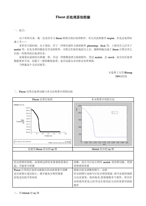
大连理工大学:Haiong2004/12/21 二、Fluent自带后处理功能与本方法将要介绍的比较Fluent自带后处理本文将要介绍的方法直接用fluent读出的xy图 Matlab绘出的xy图绘出的图形很粗,如果将这样的多条曲线重叠在一起,可能看不清楚清晰,而且可以充分利用matlab的绘图功能,得到你想要的效果Fluent自带的后处理功能做出的动画效果不清晰而且如果长宽比较大,则不能充分利用视窗好处是比较节省时间能做出较为清晰的图片,动画作出的图片动画可以充分利用视窗,将不必要的剪除方法比较笨,耗时较多,需要撑握多个软件,所以针对的使用者是已经学过在使用此方法时需要用到的软件三、用Matlab绘xy图出的文件的名字(此处为:wantmyplot,后缀默认)和选择你要保存的文件夹。
选择“所有文件”,选中wantmyplot文件,双击,出现下图:观察预览文件框里的数据,可以发现前4行为我们不需要的文本文件,因此在“导入起始行(R)”中输入“5”,点击完成。
出行如下左图:3)打开Matlab.在”Command Window”中输入”x=[]”。
4)切换到Excell窗口,按住ctrl+end,当前单元到最后一行,移动上下左右键使当前单元为A1001,如上图右图黑框。

CFDPOST后处理瞬态动画详细步骤说明
第一步:CFDPOST导入最后一步的计算dat文件结果
注意事宜:
1、FLUENT瞬态计算自动保存时,不要中途打断计算,否则导入的结果文件是
中断后到最终的计算结果(注意观察中断前后的命名不同)
2、CFDPOST导入最后一步计算结果的同时会自动导入之前所有的计算结果
第二步:创建需要做动画的云图、矢量图等(略),双击第一个时间步长的计算结果后,激活动画制作窗口
第三步:制作动画(设置循环次数1次、勾选保存动画、设置保存路径及格式),点击播放后,自动会输出动画
第四步:设置瞬态时间显示效果
将文本框中Time Value=<aa>,修改为Time =<aa>,另外你可以通过location 调整其在后处理窗口中显示的位置。
附学术沙龙简介:
“ANSYS CFD学术沙龙”平台致力于为中南地区“产学研”单位架起一条CFD 学术交流的桥梁,并积极推动“产学研”单位之间的项目合作以及尝试摸索开展人才联合培养的合作模式。
学术沙龙武汉地区CFD客户QQ群:33033610,外地CFD客户QQ群:12077406(Q群主要用于CFD软件最新资料及案例、新功能测试报告、CFD会议交流信息、CFD软件培训信息等共享)。
如果您是武汉地区流体软件使用的客户,请加入武汉地区CFD客户QQ群并在群共享内进行相关学习资料下载;如果您是外地软件使用客户,请加入外地CFD客户QQ群并在群共享内进行相关学习资料下载,加入时请输入“姓名+单位”方可通过验证。
沙龙微信公众平台:ansys_cfdsalon,欢迎您的加入,加入后第一时间了解沙龙的最新信息。

《CFD-Post 模拟后处理专题课》I 云图 I 矢量图 I 流线图 I 曲线图 I 散点图 l 数据报告 l 瞬态动 l 画高阶功能 lCFD-Post of simulation post-processing course目录CONTENTS软件简介软件启动与界面数据导入与视图操作创 建 位 置网 格 显 示体 渲 染文 本 设 置legend图例设置数据随时间的变化颗粒物Dpm模型流场涡量处理及分析(Q准则)自定义函数变量云图数据显示矢 量 图流线图与轨迹线图曲 线 图创 建 表 格软件自动化CCL基础课程小结课程简介瞬态动画效果展示模 拟 结 果 输 出多模型结果同时显示瞬态模拟动画处理3三维云图3-D 切片等值线图曲 线图网格显示点云显示创 建 线压力云图4模拟效果图展示目录CONTENTS基本操作篇软件实操篇案例操作篇高阶功能简介课程小结论1基础操作篇软件简介功能操作软件实操S e c t i o n 1.1 i n t r o d u c t i o n t o C F D -p o s t s o f t w a r e1.1节 CFD-Post 软件简介8l 软件介绍: CFD-post是一款功能强大的数据分析和可视化处理软件。
l 功能介绍:l 可以处理CFD/CFX 模拟结果显示云图、矢量图、流线图、x-y曲线图、散点图、自动出数据报告、Q准则、l 多种格式的的2-D和3-D面切片和3-D体绘图格式。
会自动输出后处理仿真报告,报告中还会包含网格、边界条件等信息,通量报告和积分计算。
三维云图3-D 切片等值线图曲 线 图9l 多结果对比:多个CFD模拟后处理文件同步对比。
l 渲 染:实现体渲染,高效显示空间分布。
l 函数功能:expression函数功能十分强大,可以自定义函数,自由输出特定模拟结果。
比如能输出压降、温度(速度)耗散等参数,可以配合FLUENT软件进行参数化及优化分析l 动画制作: 直接根据瞬时保存的数据进行动画制作;动画界面逼真。
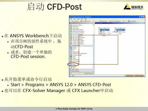
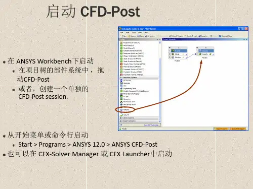
Tutorial1.Introduction to Using CFD-Post:Fluid Flow andHeat Transfer in a Mixing ElbowIntroductionThis tutorial illustrates how to use ANSYS CFD-Post to visualize a three-dimensional turbulentfluidflow and heat transfer problem in a mixing elbow.The mixing elbow configuration is encountered in piping systems in power plants and process industries.It is often important to predict theflowfield and temperaturefield in the area of the mixing region in order to properly design the junction.This tutorial demonstrates how to do the following:•Create a Working Directory•Launch ANSYS CFD-Post•Display the Solution in ANSYS CFD-Post•Save Your Work•Generate a ReportProblem DescriptionThe problem to be considered is shown schematically in Figure1.1.A coldfluid at20◦C flows into the pipe through a large inlet and mixes with a warmerfluid at40◦C that enters through a smaller inlet located at the elbow.The pipe dimensions are in inches, but thefluid properties and boundary conditions are given in SI units.The Reynolds number for theflow at the larger inlet is50,800,so theflow has been modeled as being turbulent.Note:This tutorial is derived from an existing ANSYS FLUENT case.The combination of SI and Imperial units is not typical,but follows an ANSYS FLUENT example.Because the geometry of the mixing elbow is symmetric,only half of the elbow ismodeled.Introduction to Using CFD-Post:Fluid Flow and Heat Transfer in a Mixing ElbowFigure1.1:Problem SpecificationIntroduction to Using CFD-Post:Fluid Flow and Heat Transfer in a Mixing ElbowSetupCreate a Working DirectoryCFD-Post uses a working directory as the default location for loading and savingfiles fora particular session or project.Before you run a tutorial,use your operating system’scommands to create a working directory where you can store your samplefiles and resultsfiles.By working in that new directory,you prevent accidental changes to any of the samplefiles.Copying the CAS and CDAT FilesSamplefiles are provided so that you can begin using CFD-Post immediately.You mayfind samplefiles in a variety of places,depending on which products you have:•If you have CFD-Post or ANSYS CFX,samplefiles are in<CFXROOT>\examples,where<CFXROOT>is the installation directory for ANSYS CFX.Copy the CASE andCDATfiles(elbow1.cas.gz,elbow1.cdat.gz,elbow3.cas.gz,and elbow3.cdat.gz)to your working directory.•If you have ANSYS FLUENT12:1.Download cfd-post-elbow.zip from the User Services Center(www.fl)to your working directory.Thisfile can be found by using the Documentationlink on the FLUENT product page.2.Extract the CASfiles and CDATfiles(elbow1.cas.gz,elbow1.dat.gz,elbow3.cas.gz,and elbow3.dat.gz)from cfd-post-elbow.zip to your work-ing directory.Note:–These tutorials are prepared on a Windows system.The screen shotsand graphic images in the tutorials may be slightly different than the ap-pearance on your system,depending on the operating system or graphicscard.–The case name is derived from the name of the resultsfile that you loadwith thefinal extension removed.Thus,if you load elbow1.cdat.gz thecase name will be elbow1.cdat;if you load elbow1.cdat,the case namewill be elbow1.The case names used in this tutorial are elbow1andelbow3.Introduction to Using CFD-Post:Fluid Flow and Heat Transfer in a Mixing ElbowStep1:Launch ANSYS CFD-PostBefore you start CFD-Post,set the working directory.The procedure for setting the working directory and starting CFD-Post depends on whether you will launch CFD-Post standalone,from the ANSYS CFX Launcher,from ANSYS Workbench,or from ANSYS FLUENT:•To run CFD-Post standalone,from the Start menu,right-click All Programs/ANSYS12.0/Fluid Dynamics/CFD-Post and select Properties.Type the path to yourworking directory in the Start infield and click OK,then click All Programs/ANSYS12.0/Fluid Dynamics/CFD-Post to launch CFD-Post.•ANSYS CFX Launcher1.Start the ANSYS CFX Launcher.You can run the ANSYS CFX Launcher in any of the following ways:–On Windows:∗From the Start menu,go to All Programs/ANSYS12.0/Fluid Dy-namics/CFX.∗In a DOS window that has its path set up correctly to run ANSYS CFX,enter cfx5launch(otherwise,you will need to type the full pathnameof the cfx command,which will be something similar to C:\ProgramFiles\ANSYS Inc\v120\CFX\bin).–On UNIX,enter cfx5launch in a terminal window that has its path setup to run ANSYS CFX(the path will be something similar to/usr/ansys inc/v120/CFX/bin).2.Select the Working Directory(where you copied the samplefiles).3.Click the CFD-Post12.0button.•ANSYS Workbench1.Start ANSYS Workbench.2.From the menu bar,select File/Save As and save the projectfile to the directorythat you want to be the working directory.3.Open the Component Systems toolbox and double-click Results.A Resultssystem opens in the Project Schematic.4.Right click on the A2Results cell and select Edit.CFD-Post opens.Introduction to Using CFD-Post:Fluid Flow and Heat Transfer in a Mixing Elbow•ANSYS FLUENT1.Click the ANSYS FLUENT icon()in the ANSYS program group to openFLUENT Launcher.FLUENT Launcher allows you to decide which version of ANSYS FLUENT you will use,based on your geometry and on your processing capabilities.2.Ensure that the proper options are enabled.FLUENT Launcher retains settings from the previous session.(a)Select3D from the Dimension list.(b)Select Serial from the Processing Options list.(c)Make sure that the Display Mesh After Reading and Embed Graphics Win-dows options are enabled.(d)Make sure that the Double-Precision option is disabled.You can also restore the default settings by clicking the Default button.Introduction to Using CFD-Post:Fluid Flow and Heat Transfer in a Mixing Elbow3.Set the working path to the directory created when you unzipped cfd-post-elbow.zip.(a)Click Show More.(b)Enter the path to your working directory for Working Directory by double-clicking the text box and typing.Alternatively,you can click the browse button()next to the WorkingDirectory text box and browse to the directory,using the Browse For Folderdialog box.4.Click OK to launch FLUENT.Introduction to Using CFD-Post:Fluid Flow and Heat Transfer in a Mixing Elbow5.Select File/Read/Case&Data and choose the elbow1.cas.gzfile.6.Select File/Export to CFD-Post.7.In the Select Quantities list that appears,highlight the following variables:–Static Pressure–Density–X Velocity–Y Velocity–Z Velocity–Static Temperature–Turbulent Kinetic Energy(k)8.Click Write.CFD-Post starts with the tutorialfile loaded.9.In the ANSYS FLUENT application,select File/Read/Case&Data andchoose the elbow3.cas.gzfile.10.On the Export to CFD-Post dialog,clear the Open CFD-Post option and clickWrite.Accept the default name and click OK to save thefiles.11.Close ANSYS FLUENT.Introduction to Using CFD-Post:Fluid Flow and Heat Transfer in a Mixing ElbowStep2:Display the Solution in ANSYS CFD-PostIn the steps that follow,you will visualize various aspects of theflow for the solution using CFD-Post.You will:•Prepare the case and set the viewer options•View the mesh and check it by using the Mesh Calculator•View simulation values using the Function Calculator•Become familiar with the3D Viewer controls•Create an instance reflection•Showfluid velocity on the symmetry plane•Create a vector plot to show theflow distribution in the elbow•Create streamlines to show theflow distribution in the elbow•Show the vortex structure•Use multiple viewports to compare a contour plot to the display of a variable on aboundary•Chart the changes to temperature at two places along the pipe•Create a table to show mixing•Review and modify a report•Create a custom variable and cause the plane to move through the domain to showhow the values of a custom variable change at different locations in the geometry •Compare the results to those in a refined mesh•Save your work•Create an animation of a plane moving through the domain.Introduction to Using CFD-Post:Fluid Flow and Heat Transfer in a Mixing ElbowStep3:Prepare the Case and Set the Viewer Options1.If you have launched CFD-Post from ANSYS FLUENT,proceed to the next step.For all other situations,load the simulation from the datafile(elbow1.cdat.gz)from the menu bar by selecting File/Load Results.In the Load Results File dialogbox,select elbow1.cdat.gz and click Open.2.If you see a pop-up that discusses Global Variables Ranges,it can be ignored.ClickOK.The mixing elbow appears in the3D Viewer in an isometric orientation.The wire-frame appears in the view and there is a check mark beside User Location and Plots/Wireframe in the Outline tree view;the check mark indicates that the wireframeis visible in the3D Viewer.3.Optionally,set the viewer background to white:(a)Right-click on the viewer and select Viewer Options.(b)In the Options dialog box,select CFD-Post/Viewer.(c)Set:•Background/Color Type to Solid.•Background/Color to white.To do this,click the bar beside the Colorlabel to cycle through10basic colors.(Click the right-mouse button tocycle backwards.)Alternatively,you can choose any color by clickingto the right of the Color option.•Text Color to black(as above).•Edge Color to black(as above).(d)Click OK to have the settings take effect.(e)Experiment with rotating the object by clicking on the arrows of the triad inthe3D Viewer.This is the triad:In the picture of the triad above,the cursor is hovering in the area oppositethe positive Y axis,which reveals the negative Y axis.Introduction to Using CFD-Post:Fluid Flow and Heat Transfer in a Mixing ElbowNote:The viewer must be in“viewing mode”for you to be able to click on the triad.You set viewing mode or select mode by clicking the icons inthe viewer toolbar:When you havefinished experimenting,click the cyan(ISO)sphere in thetriad to return to the isometric view of the object.4.Set CFD-Post to display objects in the units you want to see.These display unitsare not necessarily the same types as the units in the resultsfiles you load;however,for this tutorial you will set the display units to be the same as the solution unitsfor consistency.As mentioned in the Problem Description,the solution units areSI,except for the length,which is measured in inches.(a)Right-click on the viewer and select Viewer Options.The Options dialog box is where you set your preferences.(b)In the Options dialog box,select Common/Units.(c)Notice that System is set to SI.In order to be able to change an individualsetting(length,in this case)from SI to imperial,set System to Custom.Nowset Length to in(inches)and click OK.Note:•The display units you set are saved between sessions and projects.This means that you can load resultsfiles from diverse sources and always seefamiliar units displayed.•You have set only length to inches;volume will still be reported in meters.To change volume as well,in the Options dialog box,select Common/Units,then click More Units tofind the full list of settings.Step4:View and Check the MeshThere are two ways to view the mesh:you can use the wireframe for the entire simulation or you can view the mesh for a particular portion of the simulation.To view the mesh for the entire simulation:1.Right-click on the wireframe in the3D Viewer and select Show surface mesh todisplay the mesh.2.Click the“Z”axis of triad in the viewer to get a side view of the object.(Rememberthat the3D Viewer toolbar has to be in viewing mode for you to be able to selectthe triad elements.)Figure1.2:The Hexahedral Grid for the Mixing Elbow3.In the Outline tree view,double-click on User Locations and Plots/Wireframe todisplay the wireframe’s editor.Click on the Details of Wireframe editor and press F1to see help about the Wireframe object.4.On the Wireframe Details view,click Defaults and Apply to restore the originalsettings.To view the mesh for a particular portion of the simulation(in this case,the wall):1.In the Outline tree view,select the check box beside Cases/elbow1/fluid/wall,then double-click wall to edit its properties in its Details view.2.In the Details view:(a)On the Render tab,clear the Show Faces check box.(b)Select the Show Mesh Lines check box.(c)Ensure that Edge Angle is set to0[degree].(d)Click Apply.The mesh appears and is similar to the mesh shown by the previous procedure,except that the mesh is shown only on the wall.(e)Now,clear the display of the wall wireframe.In the Details view:i.Clear the Render/Show Mesh Lines check box.ii.Select the Show Faces check box.iii.Click Apply.The wall reappears.3.In the Outline tree view,clear the check box beside Cases/elbow1/fluid/wall. Note:The rest of the tutorial assumes that the wall is not visible or,if it is visible,that it is showing faces,not lines.To check the mesh:1.Select the Calculators tab at the top of the workspace area,then double-click MeshCalculator.The Mesh Calculator appears.ing the drop-down arrow beside the Functionfield,select a function such asMaximum Face Angle.3.Click Calculate.The results of the calculation appear.4.Repeat the previous steps for other functions,such as Mesh Information.Step5:View Simulation Values using the Function CalculatorYou can view values in the simulation by using the Function Calculator:1.In the Calculators view,double-click Function Calculator.The Function Calculatorappears.2.In the Functionfield,select a function to evaluate.This example uses minVal.3.In the Locationfield,select fluid.4.Beside the Variablefield,click the More Variables icon and select Volume inthe Variable Selector dialog box.Click OK.5.Click Calculate to see the result of the calculation of the minimum value of elementvolumes found in thefluid region.Note that even though the length of the elbowis measured in inches,the volume is returned in cubic meters.Step6:Become Familiar with the Viewer ControlsOptionally,take a few moments to become familiar with the viewer controls.These icons switch the mouse from selecting items in the viewer to controlling the orientation and display of the view.First,the sizing controls:1.Click the Zoom Box icon.2.Click and drag a rectangular box over the geometry.3.Release the mouse button to zoom in on the selection.The geometry zoom changes to display the selection at a greater resolution.4.Click the Fit View icon to re-center and re-scale the geometry.Now,the rotation functions:1.Click the Rotate icon on the viewer toolbar.2.Click and drag repeatedly within the viewer to test the rotation of the geometry.Notice how the mouse cursor changes depending on where you are in the viewer, particularly near the edges:Figure1.3:Orientation Control Cursor TypesThe geometry rotates based on the direction of movement.If the mouse cursor has an axis(which happens around the edges),the object rotates around the axis shown in the cursor.The axis of rotation is through the pivot point,which defaults to be in the center of the object.Now explore orientation options:1.Right-click a blank area in the viewer and select Predefined Camera/View Towards-X.2.Right-click a blank area in the viewer and select Predefined Camera/Isometric View(Z Up).3.Click the“Z”axis of triad in the viewer to get a side view of the object.4.Click the three axes in the triad in turn to see the vector objects in all three planes;when you are done,click the cyan(ISO)sphere.Now explore the differences between the orienting controls you just used and select mode.1.Click the icon to enter select mode.2.Hover over one of the wireframe lines and notice that the cursor turns into a box.3.Click a wireframe line and notice that the Details view for the wireframe appears.4.Right-click away from a wireframe line and then again on a wireframe line.Noticehow the menu changes:Figure1.4:Right-click Menus Vary by Cursor Position5.In the Outline tree view,select the elbow1/fluid/wall check box;the outer wall ofthe elbow becomes solid.Notice that as you hover over the colored area,the cursoragain becomes a box,indicating that you can perform operations on that region.When you right-click on the wall,a new menu appears.6.Click on the triad and notice that you cannot change the orientation of the viewerobject.(The triad is available only in viewing mode,not select mode.)7.In the Outline tree view,clear the elbow1/fluid/wall check box;the outer wall ofthe elbow disappears.Step7:Create an Instance ReflectionCreate an instance reflection on the symmetry plane so that you can see the complete case:1.With the3D Viewer toolbar in viewing mode,click on the cyan(ISO)sphere in thetriad.This will make it easy to see the instance reflection you are about to create.2.Right-click on one of the wireframe lines on the symmetry plane.(If you were inselect mode,the mouse cursor would have a“box”image added when you are ona valid line.As you are in viewing mode there is no change to the cursor to showthat you are on a wireframe line,so you may see the general right-click menu,asopposed to the right-click menu for the symmetry plane.)See Figure1.4.3.From the right-click menu,select Reflect/Mirror.If you see a dialog box promptingyou for the direction of the normal,choose the Z axis.The mirrored copy of thewireframe appears.If the reflection you create is on an incorrect axis,click the Undo toolbar icontwice.Step8:Show Velocity on the Symmetry PlaneCreate a contour plot of velocity on the symmetry plane:1.From the menu bar,select Insert/Contour.In the Insert Contour dialog box,acceptthe default name,and click OK.2.In the Details view for Contour1,set the following:Tab Setting ValueGeometry Locations symmetry∗Variable Velocity∗∗∗Notice how the available locations are highlighted in the viewer as you move themouse over the objects in the Locations drop-down list.You could also create a sliceplane at a location of your choice and define the contour to be at that location.∗∗Velocity is just an example of a variable you can use.3.Click Apply.The contour plot for velocity appears and a legend is automaticallygenerated.4.The coloring of the contour plot may not correspond to the colors on the legendbecause the viewer has a light source enabled by default.There are several waysto correct this:•You can change the orientation of the objects in the viewer.•You can experiment with changing the position of the light source by holdingdown the Ctrl key and dragging the cursor with the right mouse button.•You can disable lighting for the contour plot.To disable lighting,click on theRender tab and clear the check box beside Lighting,then click Apply.Disabling the lighting is the method that provides you with the mostflexibility,sochange that setting now.5.Click on the Z on the triad to better orient the geometry(the3D Viewer must bein viewing mode,not select mode,to do this).Figure1.5:Velocity on the Symmetry Plane6.Improve the contrast between the contour regions:(a)On the Render tab,select Show Contour Lines and click the plus sign to viewmore options.(b)Select Constant Coloring.(c)Set Color Mode to User Specified and set Line Color to black(if necessary,click on the bar beside Line Color until black appears).(d)Click Apply.Figure1.6:Velocity on the Symmetry Plane(Enhanced Contrast)7.Hide the contour plot by clearing the check box beside User Locations and Plots/Contour1in the Outline tree view.You can also hide an object by right-clicking on its name in the Outline tree viewand selecting Hide.Step9:Show Flow Distribution in the ElbowCreate a vector plot to show theflow distribution in the elbow:1.From the menu bar,select Insert/Vector.2.Click OK to accept the default name.The Details view for the vector appears.3.On the Geometry tab,set Domains to fluid and Locations to symmetry.4.Click Apply.5.On the Symbol tab,set Symbol Size to4.6.Click Apply and notice the changes to the vector plot.Figure1.7:Vector Plot of Velocity7.Change the vector plot so that the vectors are colored by temperature:(a)In the Details view for Vector1,click on the Color tab.(b)Set the Mode to Variable.The Variablefield becomes enabled.(c)Click on the down arrow beside the Variablefield to set it to Temperature.(d)Click Apply and notice the changes to the vector plot.8.Optionally,change the vector symbol.In the Details view for the vector,go to theSymbol tab and set Symbol to Arrow3D.Click Apply.9.Hide the vector plot by right-clicking on a vector symbol in the plot and selectingHide.CFD-Post uses the Variable setting on the Geometry tab to determine where to place objects to best illustrate changes in that variable.Once the object has been put in place, you can have CFD-Post measure other variables along those streamlines by using the Variable setting on the Color tab.In this example you will create streamlines to show theflow distribution by velocity,then recolor those streamlines to show turbulent kinetic energy:1.From the menu bar select Insert/Streamline.Accept the default name and click OK.2.In the Details view for Streamline1,choose the points from which to start thestreamlines.Click on the down arrow beside the Start From drop-down widget to see the potential starting points.Hover over each point and notice that the area is highlighted in the3D Viewer.It would be best to show how streamlines from both inlets interact,so,to make a multi-selection,click the Location editor icon.The Location Selector dialog box appears.3.In the Location Selector dialog box,hold down the Ctrl key and click velocityinlet5and velocity inlet6to highlight both locations,then click OK.4.Click Preview Seed Points to see the starting points for the streamlines.5.On the Geometry tab,ensure that Variable is set to Velocity.6.Click on the Color tab and make the following changes:(a)Set the Mode to Variable.The Variablefield becomes enabled.(b)Set the Variable to Turbulence Kinetic Energy.(c)Set Range to Local.7.Click Apply.The streamlines show theflow of massless particles through the entiredomain.Figure1.8:Streamlines of Turbulence Kinetic Energy8.Select the check box beside Vector1.The vectors appear,but are largely hidden bythe streamlines.To correct this,highlight Streamline1in the Outline tree view and press Delete.The vectors are now clearly visible,but the work you did to9.Hide the vector plot and the streamlines by clearing the check boxes beside Vector1and Streamline1in the Outline tree view.Step10:Show the Vortex StructureCFD-Post displays vortex core regions to enable you to better understand the processes in your simulation.In this example you will look at the helicity method for vortex cores,but in your own work you would use the vortex core method that youfind most instructive.1.In the Outline tree view:(a)Under User Locations and Plots,clear the check box for Wireframe.(b)Under Cases/elbow1/fluid,select the check box for wall.(c)Double-click on wall to edit its properties.On the Render tab,set Transparencyto0.75and click Apply.This makes the pipe easy to see while also making it possible to see objectsinside the pipe.2.From the menu bar,select Insert/Location/Vortex Core Region and click OK to acceptthe default name.3.In the Details view for Vortex Core Region1on the Geometry tab,set Method toAbsolute Helicity and Level to.01.On the Render tab,set Transparency to0.2.Click Apply.The absolute helicity vortex that is displayed is created by a mixture of effects fromthe walls,the curve in the main pipe,and the interaction of thefluids.If you hadchosen the vorticity method instead,wall effects would dominate.4.On the Color tab,click on the colored bar in the Colorfield until the bar is green.Click Apply.This improves the contrast between the vortex region and the blue walls.5.Right-click in the3D Viewer and select Predefined Camera/Isometric View(Y up).6.In the Outline tree view,select the check box beside Streamline1.This shows howthe streamlines are affected by the vortex regions.Figure1.9:Absolute Helicity Vortex7.Clear the check boxes beside wall,Streamline1,and Vortex Core Region1.Selectthe check box beside Wireframe.Step11:Compare a Contour Plot to the Display of a Variable on a BoundaryA contour plot with color bands has discrete colored regions while the display of a variableon a locator(such as a boundary)shows afiner range of color detail by default.The instructions that follow will illustrate a variable at the outlet and create a contour plot that displays the same variable at that same location.1.To do the comparison,split the3D Viewer into two viewports by using the ViewportLayout toolbar in the3D Viewer toolbar:2.Right-click in both viewports and select Predefined Camera/View Towards-Y.3.In the Outline tree view,double-click on pressure outlet7(which is under elbow1/fluid).The Details view of pressure outlet7appears.4.Click in the View1viewport.5.In the Details view for pressure outlet7on the Color tab:(a)Change Mode to Variable.(b)Ensure Variable is set to Pressure.(c)Ensure Range is set to Local.(d)Click Apply.The plot of pressure appears and the legend shows a smooth spec-trum that goes from blue to red.Notice that this happens in both viewports;this is because Synchronize visibility in displayed views icon is enabled.(e)Click the Synchronize visibility in displayed views icon to disable thisfeature.Now,add a contour plot at the same location:1.Click in View2to make it active,the title bar for that viewport becomes highlighted.2.In the Outline tree view,clear the check box besidefluid/pressure outlet7.3.From the menu bar,select Insert/Contour.4.Accept the default contour name and click OK.5.In the Details view for the contour,ensure that the Locations setting is pressureoutlet7and the Variable setting is Pressure.6.Set Range to Local.7.Click Apply.The contour plot for pressure appears and the legend shows a spectrumthat steps through10levels from blue to red.pare the two representations of pressure at the outlet.Pressure at the Outletis on the left and a Contour Plot of pressure at the Outlet is on the right:Figure1.10:Boundary Pressure vs.a Contour Plot of Pressure9.Enhance the contrast on the contour bands:(a)In the Outline tree view,right-click on User Locations and Plots/Contour2and select Edit.(b)In the Details view for the contour,click on the Render tab,expand the ShowContour Lines area,and select the Constant Coloring check box.Then set theColor Mode to User Specified.Click Apply.(c)Click on the Labels tab and select Show Numbers.Click Apply.10.Explore the viewer synchronization options:(a)In View1,click the cyan(ISO)sphere in the triad so that the two viewportsshow the elbow in different orientations.(b)In the3D Viewer toolbar,click the Synchronize camera in displayed views icon.Both viewports take the camera orientation of the active viewport.(c)Clear the Synchronize camera in displayed views icon and click on the Zarrow head of the triad in View1.The object again moves independently inthe two viewports.(d)In the3D Viewer toolbar,click the Synchronize visibility in displayed viewsicon.(e)In the Outline tree view,right-click onfluid/wall and select Show.The wallbecomes visible in both viewports.(Synchronization applies only to eventsthat take place after you enable the synchronize visibility function.)11.When you are done,use the viewport controller to return to a single viewport.Thesynchronization icons disappear.。
Fluent后处理第四章 Fluent后处理利用 FLUENT 提供的图形工具可以很方便的观察 CFD 求解结果,并得到满意的数据和图形,用来定性或者定量研究整个计算。
本章将重点介绍如何使用这些工具来观察您的计算结果。
1 生成基本图形在FLUENT中能够方便的生成网格图、等值线图、剖面图,速度矢量图和迹线图等图形来观察计算结果。
下面将介绍如何产生这些图形。
生成网格或轮廓线视图的步骤(1)打开网格显示面板:Display –〉Grid...图 4-1 网格显示对话框(2)在表面列表中选取表面。
点击表面列表下的 Outline 按钮来选择所有―外‖表面。
如果所有的外表面都已经处于选中状态,单击该按钮将使所有外表面处于未选中的状态。
点击表面列表下的 Interior 按钮来选择所有―内‖表面。
同样,如果所有的内表面都已经处于选中状态,单击该按钮将使所有内表面处于未选中的状态。
(3)根据需要显示的内容,可以选择进行下列步骤:1)显示所选表面的轮廓线,在图 4-1所示的对话框中进行如下设置:在Options 项选择Edges,在 Edge Type 中选择 Outline。
2)显示网格线 ,在 Options 选择 Edges,在 Edge Type 中选择 ALL。
3)绘制一个网格填充图形,在 Options 选择 Faces。
显示选中面的网格节点,在Options 选择 Nodes。
(4)设置网格和轮廓线显示中的其它选项。
(5)单击 Display 按钮,就可以在激活的图形窗口中绘制选定的网格和轮廓线。
生成等值线和轮廓的步骤:通过图 4-2 所示的等值线对话框来生成等值线和轮廓。
:Display –〉Contours...图 4-2 等值线对话框生成等值线或轮廓的基本步骤如下:(1) 在 Contours Of 下拉列表框中选择一个变量或函数作为绘制的对象。
首先在上面的列表中选择相关分类;然后在下面的列表中选择相关变量。