序列二次规划法

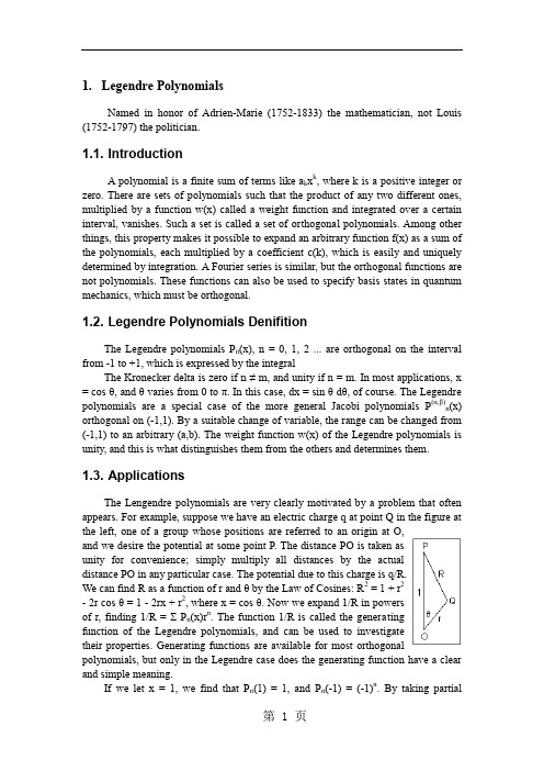
1.Legendre PolynomialsNamed in honor of Adrien-Marie (1752-1833) the mathematician, not Louis (1752-1797) the politician.1.1. IntroductionA polynomial is a finite sum of terms like a k x k, where k is a positive integer or zero. There are sets of polynomials such that the product of any two different ones, multiplied by a function w(x) called a weight function and integrated over a certain interval, vanishes. Such a set is called a set of orthogonal polynomials. Among other things, this property makes it possible to expand an arbitrary function f(x) as a sum of the polynomials, each multiplied by a coefficient c(k), which is easily and uniquely determined by integration. A Fourier series is similar, but the orthogonal functions are not polynomials. These functions can also be used to specify basis states in quantum mechanics, which must be orthogonal.1.2. Legendre Polynomials DenifitionThe Legendre polynomials P n(x), n = 0, 1, 2 ... are orthogonal on the interval from -1 to +1, which is expressed by the integralThe Kronecker delta is zero if n ≠ m, and unity if n = m. In most applications, x = cos θ, and θ varies from 0 to π. In this case, dx = sin θ dθ, of course. The Legendre polynomials are a special case of the more general Jacobi polynomials P(α,β)n(x) orthogonal on (-1,1). By a suitable change of variable, the range can be changed from (-1,1) to an arbitrary (a,b). The weight function w(x) of the Legendre polynomials is unity, and this is what distinguishes them from the others and determines them.1.3. ApplicationsThe Lengendre polynomials are very clearly motivated by a problem that often appears. For example, suppose we have an electric charge q at point Q in the figure at the left, one of a group whose positions are referred to an origin at O,and we desire the potential at some point P. The distance PO is taken asunity for convenience; simply multiply all distances by the actualdistance PO in any particular case. The potential due to this charge is q/R.We ca n find R as a function of r and θ by the Law of Cosines: R2 = 1 + r2- 2r cos θ = 1 - 2rx + r2, where x = cos θ. Now we expand 1/R in powersof r, finding 1/R = Σ P n(x)r n. The function 1/R is called the generatingfunction of the Legendre polynomials, and can be used to investigatetheir properties. Generating functions are available for most orthogonal polynomials, but only in the Legendre case does the generating function have a clear and simple meaning.If we let x = 1, we find that P n(1) = 1, and P n(-1) = (-1)n. By taking partialderivatives of 1/R with respect to x and r, and then considering the coefficients of individual powers of r, we can find a number of relations between the polynomials and their derivatives. These can be manipulated to find the recursion relation, (n + 1) P n+1(x) = (2n + 1)x P n(x) - n P n-1(x), and the differential equation satisfied by the polynomials, (1 - x2) P"n(x) -2x P'n(x) + n(n + 1) P n(x) = 0. The recurrence relation allows us to find all the polynomials, since it is easy to find that P0(x) = 1, P1(x) = x directly from the generating function, and this starts us off. The differential equation allows us to apply the polynomials to problems arising in mathematics and physics, among which is the important problem of the solution of Laplace's equation and spherical harmonics.The recurrence relation shows that the coefficient A n of the highest power of x satisfies the relation A n+1 = (2k + 1)/(k + 1) A n, and so from the known coefficients for n = 0, 1 we can find that the coefficient of the highest power of x in P n is 1.3.5...(2n-1)/n!.The polynomials can also be found by solving the differential equation by determining the coefficients of a power series substituted in the equation. This method was often used in quantum mechanics texts (see Reference 3), since the students were not usually acquainted with the mathematics of orthogonal polynomials. This method does not allow one to investigate the properties of the polynomials in any detail, however, yielding only the individual polynomials themselves.Consider the polynomials G n(x) = d n/dx n(x2- 1)n. The quantity to be differentiated is indeed a polynomial, of degree 2n, and consisting of only even powers. When differentiated n times, it becomes a polynomial of order n consisting of either all odd or all even powers of x, as n is odd or even. The coefficient of the highest power of x is 2n(2n-1)(2n-2)...(n+1), and the first two polynomials are 1 and 2x. If G(x) is substituted in the recurrence relation for the Legendre polynomials, it is found to satisfy it. If we divide G(x) by the constant 2n n!, then the first two polynomials are 1 and x. Therefore, P n(x) = (1/2n n!) d n/dx n(x2- 1)n. This is called Rodrigues's formula; similar formulas exist for other orthogonal polynomials.The great advantage of Rodrigues' formula is its form as an nth derivative. This means that in an integral, it can be used repeatedly in an integration by parts to evaluate the integral. The orthogonality of the Legendre polynomials follows very quickly when Rodrigues' formula is used. There is a Rodrigues' formula for many, but not all, orthogonal polynomials. It can be used to find the recurrence relation, the differential equation, and many other properties.For finding solutions to Laplace's equation in spherical coordinates, the Legendre polynomials are sufficient so long as the problem is axially symmetric, in which there is no φ-dependence. The more general problem requires the introduction of related functions called the associated Legendre functions that are actually built up from Jacobi polynomials, and can also be expressed in terms of derivatives of the Legendre polynomials. Physics texts generally approached the problem from first principles, never mentioning Jacobi polynomials, and thereby losing valuable insight.The Jacobi polynomials P(α,β)n(x) are orthogonal on (-1,1) with weight function w(x) = (1 - x)α(1 + x)β. Their Rodrigues' formula is P(α,β)n(x) = [(-1)n/2n n!] (1 - x)-α(1 +x)-β d n/dx n (1 - x)α+n(1 + x)β+n. The ordinary Legendre polynomial P n(x) = P(0,0)n(x). They satisfy the differential equation (1 - x2)P"(α,β)n+ [β - α - (α + β + 2)x] P'(α,β)n + n(α + β + n + 1) P(α,β)n = 0.In solving Laplace's equation by the method of separation of variables, one obtains for the θ dependence T(x), x = cos θ, the differential equationd/dx[(1 - x2)dT/dx] = [l(l+1) - m2/(1 - x2]T = 0 The substitution T(x) = (1 - x2)m/2y(x) now gives the equation(1-x2)y" - 2(m + 1)xy' + [l(l+1) - m(m+1)]y = 0, which we recognize as satisfied by the Jacobi polynomial P(m,m)l-m(x). Hence, T(x) = (1 - x2)m/2y(x) P(m,m)l-m(x). This is the associated Legendre function, often denoted P m l(x) in physics texts (e.g., Reference 4), and defined there as (-1)m(1 - x2)m/2 d m/dx m P l. The subscript is no longer the degree of the polynomial.All the above is for a positive m. Since the equation contains m2, the solution for negative m is essentially the same, except perhaps for a multiplicative factor. This is of little consequence for the traditional applications of spherical harmonics, but is critical for quantum mechanics, where relative phases matter. The choice in physics is that P-m l(x) = (-1)m[(l - m)!/(l + m)!] P m l(x), where m is always positive on the right. If you work the functions out explicitly, you will find that the functions for +m and -m are essentially the same, as might be expected, and differ at most by a factor of -1.For the same m, P m l(x) and P m l'(x) are orthogonal, and the integral of the square of P m l(x) is the same as for P l(x), multiplied by (l - m)!/(l + m)!. The functions are not orthogonal for different values of m; orthogonality of the spherical harmonics in this case depends on the φ functions.1.4. References1.M. Abramowitz and I. Stegun, Handbook of MathematicalFunctions (Washington, D.C.: National Bureau of Standards, AppliedMathematics Series 55, June 1964). Chapter 22.2. D. Jackson, Fourier Series and Orthogonal Functions(Mathematical Assoc. of America, Carus Mathematical Monographs No. 6,1941). Chapter X.3.L. Pauling and E. B. Wilson, Introduction to Quantum Mechanics(New York: McGraw-Hill, 1935). Chapter V.4.J. D. Jackson, Classical Electrodynamics, 2nd . ed. (New York:McGraw-Hill, 1975), Chapter III.2. Gauss 型积分2.1. Gauss 型求积公式的构造方法(1)求出区间[a,b]上权函数为W(x)的正交多项式pn(x)(2)求出pn(x)的n 个零点x1 , x2 , … xn 即为Gsuss 点.(3)计算积分系数2.2. 几种Gauss 型求积公式2.2.1. Gauss-Legendre 求积公式区间[-1,1]上权函数W(x)=1的Gauss 型求积公式，称为Gauss-Legendre 求积公式，其Gauss 点为Legendre 多项式的零点。

序列二次规划算法流程框图下载温馨提示:该文档是我店铺精心编制而成，希望大家下载以后，能够帮助大家解决实际的问题。

文档下载后可定制随意修改，请根据实际需要进行相应的调整和使用，谢谢!并且，本店铺为大家提供各种各样类型的实用资料，如教育随笔、日记赏析、句子摘抄、古诗大全、经典美文、话题作文、工作总结、词语解析、文案摘录、其他资料等等，如想了解不同资料格式和写法，敬请关注!Download tips: This document is carefully compiled by theeditor. I hope that after you download them,they can help yousolve practical problems. The document can be customized andmodified after downloading,please adjust and use it according toactual needs, thank you!In addition, our shop provides you with various types ofpractical materials,such as educational essays, diaryappreciation,sentence excerpts,ancient poems,classic articles,topic composition,work summary,word parsing,copy excerpts,other materials and so on,want to know different data formats andwriting methods,please pay attention!1. 初始化：设置算法参数，如最大迭代次数、收敛精度等。

选择初始点$x_0$。

(1)带约束的非线性优化问题解法小结考虑形式如下的非线性最优化问题(NLP):min f(x)「g j (x )“ jI st 彳 g j (x)=O j L其 中， ^(x 1,x 2...x n )^ R n， f : R n > R ， g j :R n > R(j I L) ， I 二｛1,2,…m ｝， L ={m 1,m 2...m p}。

上述问题(1)是非线性约束优化问题的最一般模型，它在军事、经济、工程、管理以 及生产工程自动化等方面都有重要的作用。

非线性规划作为一个独立的学科是在上世纪 50年 代才开始形成的。

到70年代，这门学科开始处于兴旺发展时期。

在国际上，这方面的专门性 研究机构、刊物以及书籍犹如雨后春笋般地出现，国际会议召开的次数大大增加。

在我国， 随着电子计算机日益广泛地应用，非线性规划的理论和方法也逐渐地引起很多部门的重视。

关于非线性规划理论和应用方面的学术交流活动也日益频繁，我国的科学工作者在这一领域 也取得了可喜的成绩。

到目前为止，还没有特别有效的方法直接得到最优解，人们普遍采用迭代的方法求解： 首先选择一个初始点，利用当前迭代点的或已产生的迭代点的信息，产生下一个迭代点，一 步一步逼近最优解，进而得到一个迭代点列，这样便构成求解( 1)的迭代算法。

利用间接法求解最优化问题的途径一般有：一是利用目标函数和约束条件构造增广目标 函数，借此将约束最优化问题转化为无约束最优化问题，然后利用求解无约束最优化问题的 方法间接求解新目标函数的局部最优解或稳定点，如人们所熟悉的惩罚函数法和乘子法；另 一种途径是在可行域内使目标函数下降的迭代点法，如可行点法。

此外，近些年来形成的序 列二次规划算法和信赖域法也引起了人们极大的关注。

在文献［1］中，提出了很多解决非线性 规划的算法。

下面将这些算法以及近年来在此基础上改进的算法简单介绍一下。

1. 序列二次规划法序列二次规划法，简称SQ 方法.亦称约束变尺度法。

序列二次规划法求解一般线性优化问题:12min (x)h (x)0,i E {1,...,m }s.t.(x)0,i {1,...,m }i i f g I =∈=⎧⎨≥∈=⎩ (1.1) 基本思想：在每次迭代中通过求解一个二次规划子问题来确定一个下降方向，通过减少价值函数来获取当前迭代点的移动步长，重复这些步骤直到得到原问题的解。

1.1等式约束优化问题的Lagrange-Newton 法考虑等式约束优化问题min (x)s.t.h (x)0,E {1,...,m}j f j =∈=(1.2)其中:,n f R R →:()n i h R R i E →∈都为二阶连续可微的实函数. 记1()((),...,())T m h x h x h x =. 则(1.3)的Lagrange 函数为： 1(,)()*()()*()mT i i i L x u f x u h x f x u h x ==-=-∑（1.3）其中12(,,...,)T m u u u u =为拉格朗日乘子向量。

约束函数()h x 的Jacobi 矩阵为：1()()((),...,())T T m A x h x h x h x =∇=∇∇.对（1.3）求导数，可以得到下列方程组：(,)()A()*(,)0(,)()T x u L x u f x x u L x u L x u h x ∇⎡⎤⎡⎤∇-∇===⎢⎥⎢⎥∇-⎣⎦⎣⎦（1.4）现在考虑用牛顿法求解非线性方程（1.4）.(,)L x u ∇的Jacobi 矩阵为：(,)()(,)()0T W x u A x N x u A x ⎛⎫-= ⎪-⎝⎭（1.5）其中221(,)L(,)()*()mxx iii W x u x u f x u h x ==∇=∇-∇∑是拉格朗日函数L(,)x u 关于x 的Hessen 矩阵.(,)N x u 也称为K-T 矩阵。

对于给定的点(,)k k k z x u =，牛顿法的迭代格式为：1k k k z z z +=+∆. 其中k k (d ,v )k z ∆=是线性方程组k k k k (,)()(x )A(x )u *()0(x )k k k k T T k k d W x u A x f A x v h ⎛⎫-⎛⎫-∇+⎛⎫= ⎪ ⎪ ⎪ ⎪-⎝⎭⎝⎭⎝⎭（1.6）的解。

文章编号：1671-7872(2023)03-0313-11基于序列二次规划算法的插电式混合动力汽车模型预测控制策略张代庆 ，俞　聪 ，牛礼民 ，汪　恒 ，张义奇(安徽工业大学 机械工程学院, 安徽 马鞍山 243032)摘要：为提升插电式混合动力汽车(PHEV)的车速预测精度和燃油经济性，提出基于序列二次规划(SQP)算法的模型预测控制能量管理策略。

以卷积神经网络(CNN)构建的车速预测模型为基础，选取三类典型历史工况数据作为CNN 车速预测模型的训练集，使用鲸鱼优化算法(WOA)优化CNN 参数，通过优化的WOA-CNN 模型预测未来时域内的车速；采用SQP 算法对模型预测控制策略进行求解，且与基于规则的电量消耗和电量保持(CD-CS)策略和基于全局优化的动态规划(DP)策略的控制结果进行对比分析，验证所提策略的有效性。

结果表明：通过WOA-CNN 模型可提高车速预测精度，为4.88%~8.39%；与DP 控制策略相比，本文提出策略的燃油消耗量高出1.98%，但计算时间减少了74.32%，能量管理的实时性得到大幅提升；与CD-CS 控制策略相比，提出策略的节油率为20.37%。

综合考虑，本文提出策略的整车能量消耗和计算成本较优，可合理实现对PHEV 转矩分配的智能控制。

关键词：能量管理策略；模型预测控制；卷积神经网络；鲸鱼优化算法；序列二次规划；混合动力汽车中图分类号：U 469.72 文献标志码：A doi ：10.12415/j.issn.1671−7872.22264Predictive Control Strategy of PHEV Model Based on Sequential QuadraticProgramming AlgorithmZHANG Daiqing, YU Cong, NIU Limin, WANG Heng, ZHANG Yiqi(School of Mechanical Engineering, Anhui University of Technology, Maanshan 243032, China)Abstract ：In order to improve the speed prediction accuracy and fuel economy of plug-in hybrid electric vehicle (PHEV), a model predictive control energy management strategy based on sequential quadratic programming (SQP)algorithm was proposed. Based on the speed prediction model constructed by convolutional neural network (CNN),three types of typical historical working conditions were selected as the training set of CNN speed prediction model.Whale optimization algorithm (WOA) was used to optimize CNN parameters, and the optimized WOA-CNN model was used to predict the future speed in the time domain. SQP algorithm was used to solve the model predictive control strategy, and the control results with the rule-based charge depleting and charge sustaining (CD-CS) control strategy and the global optimization based dynamic programming (DP) control strategy were compared and analyzed to verify the effectiveness of the proposed strategy. The results show that the prediction accuracy of vehicle speed收稿日期：2022-10-24基金项目：先进数控和伺服驱动技术安徽省高校重点实验室开放基金项目(XJSK202104)；安徽工程大学电力驱动与控制安徽省重点实验室开放基金项目(DQKJ202204)；安徽省大学生创新创业项目(S202110360259)作者简介：张代庆(1997—)，男，黑龙江大庆人，硕士生，主要研究方向为新能源汽车控制技术。

科技与创新┃Science and Technology&Innovation ·116·2023年第17期文章编号：2095-6835（2023）17-0116-03船舶定位系统推力分配方法及策略研究余祥（安徽省淮河船舶检验局，安徽蚌埠233000）摘要：随着科技的发展，海洋资源的勘探、开发和利用从浅海拓展至深海。

在这种情况下，船舶动力定位和推力分配成为了船舶工程领域的研究热点。

动力定位系统是利用船舶或平台自身推进器产生的推力来抵消外部环境力的技术，以维持预定位置或轨迹[1]。

推力分配模块是该系统的关键组成部分，其主要功能是在有限时间内找到最优的推力和角度组合，以满足控制器对合力和力矩的要求。

首先，总结了国内外动力定位系统中推力分配的研究现状，并说明研究的目标；其次，引入了数学模型，以优化推力分配，该数学模型包括目标函数和约束条件；最后，介绍了2种不同的数学优化算法，即二次规划（Quadratic Programming，QP）算法和序列二次规划（Sequential Quadratic Programming，SQP）算法，并将它们应用于推力分配问题数学模型的求解[2]。

此外，还介绍了一种自适应组合偏置算法，该算法能够根据控制力的大小和方向自适应地调整偏置量的大小及全向推进器的组合方式。

关键词：动力定位；推力分配；数学模型；组合偏置算法中图分类号：U664.82文献标志码：A DOI：10.15913/ki.kjycx.2023.17.034船舶动力定位系统（Dynamic Positioning System，DP）是利用船舶自身设备和先进技术实现船舶在海上进行自主控制的技术[3]。

传统的推力分配方法无法考虑到海洋环境的变化和复杂性，不能实现最优的推力分配，从而影响了DP系统的性能和船舶的操作效率[4]。

推力分配方法和策略的研究可以为船舶动力定位系统的发展提供技术支持和理论指导，提高船舶的定位精度和控制效率，进一步提升海洋工程的安全性和可靠性。