清华弹性力学课件_Elasticity of Solids
- 格式:ppt
- 大小:2.30 MB
- 文档页数:45


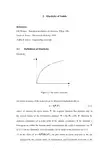
2.Elasticity of SolidsReferencesJ.H.Weiner ,Statistical mechanics of elasticity, Wiley, 1981Green & Zerna ,Theoretical elasticity, 1968Ashby & Jones ,Engineering materials2.1 Definition of Elasticity ElasticityσFFigure 2.1 An elastic response.An elastic response of the material can be abstracted mathematically as()X F ,T σ= (2.1) where σ denotes the stress tensor, T the response function that depends only on the current values of the deformation gradient X x F ∂∂=, with X denoting the material coordinates of a point while x the spatial coordinates. If the material is homogeneous within the domain under consideration, the explicit dependence on X in (2.1) can be eliminated. Several remarks can be made to the definition in (2.1):(1) In the claim of ()()X t X,F ,T σ=, one pins down an elastic response as the one prtrayed by the current status of deformation, and henceforth irrelevant to thehistory or the process of deformation. The strain rate plays no role in the constitutive response. A hysteresis is ruled out, as shown in Fig. 2.1. Whenever the loading is removed, the original configuration (or the “non-distorted configuration”) is recovered.(2)For the special case of infinitesimal deformation, the response (2.1) is reduced to()X,εσ=, where εdenotes the strain tensor. The response function T is not Tnecessarily linear.(3)For homogeneous materials, one has ()Fσ=in finite deformation andT()εσ=for infinitesimal deformation.T(4)For the even special case of infinitesimal deformation, homogeneous material andlinear elasticity, the generalized Hooke’s law ε=is recovered, with Cσ:Cbeing the fourth-rank stiffness tensor. The notations of C as the stiffness tensor and S as the compliance tensor, not the otherwise according to their initials, unfortunately became the convention in the historic development of elasticity.The difference between the material responses at a solid state and a fluid state can be quoted as follows (Mechanics of Solids, The New Encyclopedia of Britannica, 15th edition, V ol. 23, pp. 734-747, 2002, written by J. R. Rice):“A material is called solid rather than fluid if it can also support a substantial shearing force over the time scale of some natural process or technological application of interest.”An elastic solid can resist the volume and shape changes, whereas a fluid can only resist the volume change but not the shape changes in a relatively long time scale. HyperelasticityHyperelasticity refers to an elastic response that can be defined by a potential. The basic assumptions are: (1) the response of the elastic body only depends on its current state, not the processes to achieve it; and (2) the current state of the elastic body can be described by a tensor, such as the strain tensor εfor the special case of infinitesimal deformation. The first assumption leads to the independence ofdeformation paths. It was the great mathematician Green who first exploited that condition to arrive the path independent condition of a multi-dimensional integration. The elasticity so-defined was called Green elasticity. As the readers may recall from their calculus course, such a path independency leads to the Green ’s conditions among partial derivatives of the integrands, and the existence of a potential function. We denote this elastic potential as W that has the physical significance of the elastic energy stored within the body. A hyperelastic constitutive response is thenij ij W εσ∂∂=. (2.2)That is also valid for non-linear elastic response. For a linear elastic material, one has kl ij ijkl C W εε21=. (2.3) The combination of (2.2) and (2.3) leads to the generalized Hooke ’s lawkl ijkl ij ij C W εεσ=∂∂= (2.4)2.2 Two Physical Origins of ElasticityThe elasticity of a solid may depend on other things beside the deformation state. For example, temperature and disorder status in the material structure may influence the elastic response. The influences from these factors are often material specific and they may get quite intricate. In terms of the temperature effect, a crystalline solid expands or shrinks when temperature rises or falls; while a polymeric solid, such as a rubber band, shrinks upon heating. These opposite behaviors come from different physical origins of elasticity that will be addressed briefly in this section. The book of J.H. Weiner is referred for the in-depth understanding.Energetic and Entropic StressesThe Helmholtz free energy H of a solid can be expressed asST U H -= (2.5) where U denotes the internal energy, S the entropy, and T the absolute temperature in Kelvin. The internal energy of an elastic material excluding the thermal fluctuation energy ST gives the Helmholtz energy that can be freed. Similar to the simplifiedversion of hyperelastic relation (2.2), the stress tensor can be deduced asij ij ij ij S T U H εεεσ∂∂-∂∂=∂∂=. (2.6)A Maxwell relation can be derived asT S ij ij ∂∂=∂∂σε. (2.7) Accordingly, (2.6) may have an alternative presentationT T U ij ij ij ∂∂-∂∂=σεσ (2.8) Figure 2.2 shows a graphical interpretation of (2.8). The total stress ij σ is composed of two terms: the energetic stress ijU ε∂∂ and the entropic stress T T ij ∂∂-σ.T -T Figure 2.2 Energetic and entropy stresses.Consider the stress versus the temperature curve above. At a prescribed temperature T , the corresponding stress is composed of two parts, the entropy stress denotes the interval between the horizontal line and the tangent extrapolated to the absolute zerotemperature, and the energetic stress for the remaining part. For a perfect crystal, the energetic stress dominates; for an amorphous polymer, the entropy stress dominates. These extreme cases will be discussed below to explore two physical origins of elasticity.CrystalsA crystal is built by periodic repetition of its unit cell. The primary bonding in the unit cell can be ionic, covalent or metallic. The bonding can be isotropic (such as metallic bonds) or polarized (such as the covalent and ionic bonds). Those bonds typical melt at a temperature (related to the kinetic energy of the atoms) range between 1000-5000K. The secondary bonding is composed by Van der Walls and hydrogen bonds, and they have a much lower range (100-500K) of melting point.The bonding between two atoms is described by an inter-atomic potential U (Fig. 2.3). The bonds can simplified as springs connecting the neighboring atoms, as shown in Fig. 2.3. The spring-like inter-atomic bonding provides a physical origin for the elasticity of a crystalline solid.bond energy UFigure 2.3 Spring-like inter-atomic bonding (above) and inter-atomic energy curve(below).The inter-atomic force F is given by the derivative of U with respect to the inter-atomic distance r . A plot of the inter-atomic force is given in Fig. 2.4. The location where d U /d r vanishes refers to an equilibrium location of the atom, marked by an inter-atomic distance of 0r . The force is repulsive when 0r r < and attractive when 0r r >. The stiffness of the bonding spring equals to the second derivative ofthe inter-atomic potential with respect to the distance, 22drU d S =. The maximum inter-atomic force occurs at the location where S vanishes, as shown in Fig. 2.4. The value of S at the equilibrium location0220r r dr U d S =⎪⎪⎭⎫ ⎝⎛= (2.9)relates to the elasticity of the linear Hooke ’s law.FF Figure 2.4 Inter-atomic force.The elasticity tensor of a crystalline solid depends on the orientation, as the consequence of the atomic arrangement in the form of a lattice, which is spanned by the periodic repetition of a unit cell. For a simple cell, this repetitive construction of the crystal lattice is mathematically represented by the following specification on the atom sites332211321a a a r n n n n n n ++= (2.10) where i n (3,2,1=i ) are integers, and i a (3,2,1=i ) are lattice vectors that are not necessarily mutually perpendicular. The lattice formed by (2.10) has a translational symmetry.For a composite cell, the representation (2.10) is replaced byi i n n n n a r =321, ξa r +=i i n n n n 321' (2.11) Summation convention is implied for repeated indices. An example for a material of composite cell is grapheme and nanotubes.Aside from the translational symmetry, a crystal lattice can be categorized by various types. A generally accepted notion is the classification of Bravais lattices. The seven Bravais lattices are tri-clinic, mono-clinic, orthogonal, rhombohedral, tetragonal, hexagonal and cubic. The symmetry derived by these lattices can be characterized bythe group theory, via 32 point groups and 236 space groups. Their implications to the elasticity tensor will be explored in Section 2.4.Long Chain PolymersWe next turn to the elasticity of long chain polymers, a scientific wonder that was shaped in the first half of the 20th century by the famous scientists such as Mark, James, Guth and Flory.The long-chain polymers, such as rubbers, are highly elastic in terms of large extensibility and low elastic modulus. They are nearly incompressible. A strange feature of polymeric materials is the Gough-Joule effect: they shrink during heating and expand during cooling. Long chain polymers can be heated up rapidly during adiabatic deformation. You can test this phenomenon by fast pulling a rubber band and feeling it on your lip.These bizarre mechanical behaviors come from the unique microstructure of long chain polymers, and the latter manifests in terms of the entropy stress. Figure 2.5 depict the structure. A polymer is formed by the backbone connected by taunt covalent bonding attached with the tangling sidegroups formed by much weaker bonding. Neither the bonding length nor the bonding angle of the backbone can be changed appreciably. The sidegroups are used to form weak interaction, such as the van der Waals type, among the neighboring chains. A rotational degree of freedom, however, exists between the neighboring links in the backbone. That grants the polymer chain certain degree of flexibility for the actual shape of its backbone.(strong covalent bond)(weak bond)Figure 2.5 Long chain structure of polymeric solid.Consider a backbone connected by n links where n is a large number for the macromolecule. Two end points of the chain form a distance vector R . Under a fixed vector R , there are many ways for the polymer chain to arrange itself, as shown in Figure 2.6.Under a fixed number n for the links of the chain and a fixed end-to-end distance R , the number of possible arrangement, denoted by ()n W W ,R =, can be computed by the model of random walking. The same model was used by Albert Einstein in theoretical physics calculation. The number of possible arrangement of many polymer chains obeys a Gaussian distribution()⎪⎪⎭⎫ ⎝⎛-⎪⎭⎫ ⎝⎛=2223223exp 23,nb R nb n W πR , R =R (2.12) where b denotes the effective length of freely jointed links, or the step size of the random walk. For a freely jointed polymer chain, one has a b =; the length increase to a b 2= for freely rotating chain as shown in the lower graph of Fig. 2.5; and it becomes a b 7.6=for poly-ethelene.R ~Figure 2.6 Arrangement for a long chain polymeric to achieve a certain end to enddistance.Under a fixed n , the longer the distance R , the smaller the number of the possible arrangements. Subjected the polymer to a strain ε so that the vector r R →. That change provokes a related change of W . An elongation decreases the amount of W whilst a contraction increases it. The number of the possible arrangements W of n links in the chain and its stress response can be bridged by Boltzmann ’s formula for configuration entropy in statistical mechanics. That links the configuration entropy q S with W byW K S B q ln = (2.13) where B K is the famous Boltzmann constant. The total entropy of the system is composed of the configuration entropy q S and the vibration entropy S p , while the latter hardly changes during the deformation. The entropy stress, namely the second term in (2.6) can be computed asij Bij q ij W W T K S T S T εεε∂∂-=∂∂-≈∂∂- (2.13)The physical origin for rubber elasticity is revealed: the stress is caused by the reduction of the configuration entropy due to elongation.By means of the network model, James and Guth (1947) were able to derive the following elastic response for rubber-like polymers in uniaxial tension:()2--=λλσT NK B (2.14) where λ denotes the stretching ratio, and N the number of links per unit volume. The elastic law of (2.14) is referred as the Neo-Hookeian law in rubber elasticity.1234567812340λσFigure 2.7 Rubber elasticity: theory and experiment.Figure 2.7 plotted the experimental curve, decorated by circles, of rubber-like polymer undergoing stretch up to 8-folds of its original length. The Neo-Hookeian prediction (2.14) agrees with the experiment at the beginning, but two noticeable deviations occur in the later stage of elongation. For a stretching ratio between 2 and 5, the Neo-Hookeian law seems to overestimate the stress response. This effect was first corrected by Mooney, and called thereafter as the Mooney effect. The Mooney-Rivlin constitutive relation developed later can follow this deviation. For a stretching ratio higher than 6, the Neo-Hookeian prediction underestimate the stress response. Two explanations were offered for the upturn of the stress response: one due to the crystallization of polymers under large elongation, and the other due the non-Gaussian chain theory.2.3 Tensor Description of ElasticityVoigt SymmetryRecall the linear elastic response (2.4), namely kl ijkl ij C εσ=. All components of the fourth-rank elasticity tensor ijkl C can be measured from tests involving only homogeneous deformation. For a three-dimensional problem, all indices i , j , k and lmay have 3 possible numbers. That gives the maximum possible combinations of indices as 8134=.We now try to find ways to eliminate the unnecessary tests for a complete characterization of the stress tensor. First consider the symmetries of the stress and the strain tensors. For infinitesimal deformation, the strain tensor is given by a symmetric expression of ()ji i j j i ij u u εε=+=,,21. The anti-symmetric part, the rotation, bears no effect on the stress response. On the other hand, the reciprocal law of shear stresses (ji ij σσ=) derived by neglecting the couple acting on a body element gives rise of a symmetric stress tensor. We now use these symmetry requirements to derive the corresponding conditions for the elasticity tensor.First consider the stress symmetry ji ij σσ=. Substituting this condition to (2.4), one has kl jikl kl ijkl C C εε=, kl ε∀. Accordingly, one has the inter-changeability of the first two indices of the elasticity tensorjikl ijkl C C =Next consider the strain symmetry lk kl εε=. Equation (2.4) can be rearranged askl ijlk lk ijlk kl ijkl C C C εεε==, kl ε∀. That leads to the inter-changeability of the last two indices of the elasticity tensorijlk ijkl C C =Linear elasticity is a special case of hyperelasticity as described at the end of Section 2.1. An elastic potential kl ij ijkl C W εε21= exists as the strain energy density. Equation (2.2), ijij Wεσ∂∂=, leads to klij klij ijkl WC εεεσ∂∂∂=∂∂=2 In an Euclidian space, the order of differentiations bears no effect. One then concludes the interchangeability between the first two and the last two indices of the elasticitytensor:klij ijkl kl ij ijklC W W C =∂∂∂=∂∂∂=εεεε22 The above symmetry requirement can be summarized asklij ijlk jikl ijkl C C C C ===(2.15)They are called the V oigt relation of the elasticity tensor. Matrix RepresentationDue to the V oigt symmetry, it is frequently to represent the fourth rank of the elasticity tensor by a symmetric 66⨯ matrix, the elasticity matrix. The matrix is sequenced to put the 6 independent components of a symmetric second order tensor in the counter-clockwise manner described below.Therefore, the fourth rank symmetric elasticity tensor is transformed into the following symmetric elasticity matrix[]⎥⎥⎥⎥⎥⎥⎥⎥⎦⎤⎢⎢⎢⎢⎢⎢⎢⎢⎣⎡=⇒665655464544363534332625242322161514131211C C C C C C C C C C C C C C C C C C C C C C ijklαβC (2.16)with j i --=9α and l k --=9β. The general anisotropy refers to the case where 21 elastic constants in (2.16) are totally unrelated. A material example for such a general anisotropy is the triclinic crystals whose three lattice vectors have different lengths, namely 321a a a ≠≠, and neither two of them is mutually perpendicular. The elastic strain energy for such a case could be in arbitrary quadratic form of the six⎥⎥⎥⎥⎥⎥⎦⎤⎢⎢⎢⎢⎢⎢⎣⎡↑↑←342561⎥⎥⎥⎥⎥⎥⎥⎥⎦⎤⎢⎢⎢⎢⎢⎢⎢⎢⎣⎡↑↑←)23()13(333231)12(232212131211symmetric components of strain, namely()231312332211,,,,,21εεεεεεεεW C W kl ij ijkl ==(2.17)Most natural or technical materials have a certain degree of symmetries. The implication of these symmetry to the reduction of the elastic constants will be revealed below. Coordinate Transform1XFigure 2.8 Coordinate transform.Consider an affine transformation from coordinates i x to coodinates i x , as shown in Fig. 2.8. The components of the second rank strain tensor and the fourth order elasicity tensor in the new coordinates with superimposed bars areij j s i r rs x x x x εε∂∂∂∂=, ijkl ltk p j s i r rspt C x x x x x x x x C ∂∂∂∂∂∂∂∂=(2.18)Reflective SymmetryA reflective symmetry refers to the invariance of material property with respect to a coordinate plane such as 03=x . It can be equally represented by rotating the x 3 axis of 180o . Consider the following coordinate transformationααx x =, 33x x -=, (α=1,2).(2.19)Denote ij δ as the Kronecker Delta, whose diagonal elements are equal to unity and the off-diagonal ones equal to zero. That givesr r x x ααδ=∂∂ and r r x x33δ-=∂∂. According to the first expression of (2.18), the strain components in the new coordinates areαβαβεε=,3333εε=,33ααεε-=(2.20)If the elastic properties of the material is invariant with respect to a mirror reflection of 03=x , then the strain energy cannot be any arbitrary functions of the strain components, but has to be restricted to the following form()231222321312332211,,,,,,εεεεεεεεW W =(2.21)That implies any quadratic terms related to 13ε and 23ε in the strain energyexpression may only take the form of 213ε, 223ε and 2312εε. Consequently, anyelastic constants related to the cross products between the components()12332211,,,εεεε and the components ()2313,εε should vanish. The elastic matrix isreduced to:[]⎥⎥⎥⎥⎥⎥⎥⎥⎦⎤⎢⎢⎢⎢⎢⎢⎢⎢⎣⎡=6655454436332623221613121100000000C C C C C C C C C C C C C C (2.22)Only 13 elastic constants are present for a material with one reflective symmetry. If the material possesses a further reflective symmetry with respect to a second orthogonal coordinate plane, say the plane of 01=x , the response of the material would remain the same under the following coordinate transform:11x x -=,22x x =,33x x -=(2.23)It is a straightforward matter to deduce that the elastic strain energy would possess a more restricted form of()223213212332211,,,,,εεεεεεW W = (2.24)Its dependences with terms such as 2313εε, 1112εε, 2212εε and 3312εε are ruled out. The elasticity matrix for such a material has the following form[]⎥⎥⎥⎥⎥⎥⎥⎥⎦⎤⎢⎢⎢⎢⎢⎢⎢⎢⎣⎡=665544332322131211000000000000C C C C C C C C C C (2.25)It has 9 independnt elastic constants, and is called orthotropic. Examples of such materials include crystals of orthogonal lattice, and cross-ply composite laminates. Rotation SymmetryThe elastic response for a certain material may remain invariant when rotating it about a symmetry axis by a specific angle. Such a symmetry is called a rotation symmetry. The reflective symmetry discussed above corresponds to two-fold rotation symmetry, or symmetry to a rotation of 180 degrees. Without loss of generality, we label the symmetry axis as 3x , an arbitrary rotation about that axis is given by the following coordinate transformation:ωωsin cos 211x x x +=, ωωcos sin 211x x x +-=, 33x x =(2.26)The cases of the rotation angels of 0180=ω, 0120=ω, 090=ω and 060=ω are termed rotation symmetries of 2-folds, 3-folds, 4-folds and 6-folds, respectively. Transverse IsotropyIf a solid maintains its elastic response by rotation an arbitrary angle with respect to an aixs, the solid is termed transversely isotropic. In the coordinate transformation stated in (2.26), the following relations always hold for an arbitrary value of ω:22112211εεεε+=+, 21222112122211εεεεεε-=-, 223213223213εεεε+=+, ij ij εε= (2.27) where ij ε denotes the determinant of the strain tensor. Relations in (2.27) are called the invariance relations under the rotation transform (2.26). It can also show that the relations in (2.27) are the only ones invariant at any values of ω.If the material under consideration possesses the transverse isotropy, its elastic strain energy can only be the function of these strain invariants. Consequently, it has to be ina form of ()3322321321222112211,,,,εεεεεεεεεij W W +-+=. The only possible quadratic terms in strain components are ()22211εε+, 2122211εεε-, 223213εε+, 233ε and ()332211εεε+. Therefore, only 5 independent elastic constants exist. The elastic matrixis reduced to:[]()⎥⎥⎥⎥⎥⎥⎥⎥⎦⎤⎢⎢⎢⎢⎢⎢⎢⎢⎣⎡-=221144443313111312112100000000000C C C C C C C C C C C (2.28)Examples for this class of materials include the wood and bamboo in nature, the pole vault in sport, and the man made composite materials reinforced by uni-directional fibers. IsotropyWe finally examine the most special materials that are isotropic in their elastic response. A typical example of such materials is a polycrystal composed of grains with complete random orientations. Consider an arbitrary rotation ij R on the coordinates such as j ij i x R x =. The rotation tensor obeys the relation of1R R =⋅T or ik jk ij R R δ=(2.29)Due to the second expression of (2.18), the elastic tensor in an arbitrarily rotated coordinates is ijkl tl pk sj ri rspt C R R R R C =. The only possibility for rspt C so defined to be invariant under arbitrary rotation is the following formjk il jl ik kl ij ijkl C δδμδμδδλδ'++=.Furthermore, the symmetry with respect to indices i and j implies 'μμ=. One then arrives at the elastic tensor for an isotropic material()jk il jl ik kl ij ijkl C δδδδμδλδ++=(2.30)Only two independent elastic constants λ and μ are encountered in (2.30) for anisotropic material. They are termed the Lamè constants. Substituting (2.30) into (2.4), one obtains the following generalized Hooke ’s law:ij kk ij ij μεελδσ2+=(2.31)Simple ShearWe now consider the generalized Hooke ’s law for three particular cases: simple shear, radial dilation, and uniaxial tension. The case of simple shear will be discussed first, as shown in Fig. 2.9.The kinematics given in Fig. 2.9 can be described by 21x u γ= and 032==u u . Consequently, all strain components are zero except 2/12γε=, where γ is the shear amount. The generalized Hooke ’s law leads to a shear stress of μγσ=12, while the other stress components are absent. The physical meaning of the second Lamè constant μ now becomes transparent: it is the shear modulus of the material.Figure 2.9 Simple shear.DilationNext consider dilatation in radial direction. The radial dilation adopts a kinematical field of i i x u 3θ=. That delivers a spherical strain tensor of ij ij δθε3=, where kk εθ=symbolizes the volume dilation. The generalized Hooke ’s law (2.31) becomes ij ij K θδσ=(2.32)whereμλ32+=K (2.33)denotes the bulk modulus of the material by (2.32). The stress tensor presented in (2.32) is spherical. In the general case, we can always decompose the stress and strain tensors into the spherical and deviatoric (traceless) parts as follows:ij kkij ij S δσσ3+=, ij kkij ij e δεε3+=.(2.34)It is a straightforward matter to show that 0=kk S and 0=kk e . The decomposition (2.34) suggest another representation of the generalized Hooke ’s law asij ij e S μ2=, kk kk K εσ3=(2.35)The strain energy density can be explicitly expressed as221814121kk ij ij kk ij ij KS S K e e W σμεμ+=+= (2.36)Uniaxial TensionOur last example concerns uniaxial tension where the only non-trivial stress component is σσ=11. The generalized Hooke ’s law (2.31) can be inverted as⎪⎭⎫⎝⎛-=ij kk ij ij K δσλσμε321 (2.37)by utilizing the relation (2.33). Take the “11”, “22”, and “33” components of the above equation, one hasσσλμεEK 1312111≡⎪⎭⎫ ⎝⎛-=, σσμλεεE v K -≡-==63322, (2.38)where the Young ’s modulus and the Poisson ’s ratio are given byμμ+=K K E 39, μμ+-=K K v 32321,(2.39)Among 5 symbols for elastic response, namely the Young ’s modulus E , the Poisson ’s ratio v , the shear modulus μ, the bulk modulus K and the first Lamè constant λ, any one of them can be expressed by any two others.2.4 Physical Foundation of Elastic SymmetryCrystals and Bravais LatticesThe elastic symmetry in a perfect crystal is motivated by its lattice structure. Table 2.1 lists 7 Bravais lattices, along with their corresponding symmetry groups and the number of independent elastic constants.Table 2.1 Seven Bravais LatticesLattice type Symmetry group Elastic constantstriclinic null (center symmetry)21 mono-clinic 2-fold rotation13 orthogonal two orthogonal 2-fold rotations9 tetragonal 4-fold rotation 7 rhombohedral 3-fold rotation 9 hexagonal 6-fold rotationcubic four 3-fold rotations about the cube diagonalsCauchy ’s RelationThe great mathematician Cauchy explored the physical foundation of a elastic crystal 180 years ago. His formulation led to the so-called Cauchy ’s relation for elastic constants. For the elasticity tensor ijkl C , the V oigt symmetry (2.15) indicates the interchangeabilities of the following index groups(i ,j )↔(j ,i ), (k ,l )↔(l ,k ), (i ,j )↔(k ,l )while the Cauchy ’s symmetry adds the interchangeability of(j ,l )↔(l ,j ).That grants the complete symmetry of an elastic tensor. For the general anisotropic materials (such as tri-clinic crystal), the Cauchy ’s symmetry adds 6 additional relations for the components of elastic matrix5614C C =, 6612C C =, 5513C C =, 4536C C =, 4423C C =, 4625C C = (2.40)Therefore, only 15 independent elastic constants are allowed for a generallyanisotropic material provided the Cauchy ’s symmetry holds.Central Force Assumption of CauchyCauchy derived his relation among elastic constants based on an assumption that the interaction among the atoms were in the form of central forces of any atom pairs. As shown in Fig. 2.10, a vector linking atom l and atom l ’ is denoted as ()()()l x l x l l x i i i -=∆'',, whose length can be computed as ()()()',',',2l l x l l x l l R i i ∆∆=. The change in that distance by imposing a strain tensor ij ε is()()()()()',',2',',22l l x l l x l l R l l r j i ij ij ∆∆+=-εδ (2.41) Cauchy assumed that the inter-atomic potential U depended only on the distances of various pairs of atoms in the aggregate, namely()()∑=','',l l ll l l r U ϕ(2.42)where 'll ϕ denotes the interaction energy between atom l and atom l ’, with l and 'l taking values in all atoms within the lattice. Generalizing (2.9) for the three-dimensional case, one can compute the elastic constants from the second derivatives of the inter-atomic potential as ()()()()()()()',',',',',',41',2'22l l x l l x l l x l l x l l r l l r V U V C l k j i l l oll okl ij ijkl ∆∆∆∆∂∂=∂∂∂=∑ϕεε. (2.43) l'lFigure 2.10 Interaction between two atoms.Expression (2.43) indicates that indices l k j i ,,, can switch their orders arbitrarily。


弹塑性力学第四章 弹性力学的基本方程与解法一、线性弹性理论适定问题的基本方程和边界条件对于在空间占有体积域V 的线弹性体在外加恒定载荷和固定几何约束条件下引起的小变形问题,若以, ,u εσ作为求解变量,则可以建立如下偏微分方程边值问题: 几何方程()1,,2ij i j j i u u ε=+ ()12∇+∇u u ε= (1a)广义胡克定律 ij ijkl kl E σε= :E σ=ε(1b)平衡方程 ,0ij j i f σ+= ∇⋅+=f 0σ V∀∈x (1c)以上方程均要求在域内各点均满足。
边界条件 u u i i = ∀∈x S ui (2a)n t j ji i σ= ∀∈x S ti(2b)对于适定问题,即不仅要求保证解存在唯一,而且有较好的稳定性。
当载荷或边界条件给定值有微小摄动时,应能保证问题解的变化也是微小的。
对于边界条件的提法就有严格的要求。
即要求:S S S S S ui ti ui ti U I ==∅(2c)对于各向同性材料,其广义胡克定律可具体写成 σλεδεij kk ij ij G =+2 ()tr 2G λ+I σ=εε (3a)()11ij ij kk ij E ενσνσδ⎡⎤=+−⎣⎦ ()()1tr Eνν=⎡⎤⎣⎦I ε1+σ−σ (3b)以上就域内方程来说,一共是对于u ,,σ ε的15个独立分量u i ij ij ,, σε的15个方程。
对于边界条件来说,三维问题每点有三个边界条件,而且是在三个正交方向上每个方向有一个边界条件,这个边界条件或者给定位移、或者给定面力。
这三个正交第四章 弹性力学的基本方程与解法方向可以是整体笛卡儿坐标系的三个方向,也可以是边界自然坐标系的三个方向(即法向和两个切向)。
从更一般来说,除去给定位移或面力外,还有另一种线性的边界条件t K u c i ij j i +=(4)这是一种弹性约束条件。
用这个条件可以取代给定位移或给定面力的条件。