伍德里奇计量经济学导论第四版
- 格式:pdf
- 大小:89.09 KB
- 文档页数:3

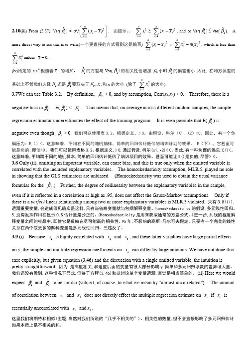
2.10(iii) From (2.57), Var(1ˆβ) = σ2/21()n i i x x =⎛⎫- ⎪⎝⎭∑. 由提示:: 21n i i x=∑ ≥21()n i i x x =-∑, and so Var(1β ) ≤ Var(1ˆβ). A more direct way to see this is to write(一个更直接的方式看到这是编写) 21()n ii x x =-∑ = 221()n i i x n x =-∑, which is less than21n i i x=∑unless x = 0.(iv)给定的c 2i x 但随着x 的增加, 1ˆβ的方差与Var(1β )的相关性也增加.0β小时1β 的偏差也小.因此, 在均方误差的基础上不管我们选择0β还是1β 要取决于0β,x ,和n 的大小 (除了 21n i i x=∑的大小).3.7We can use Table 3.2. By definition, 2β > 0, and by assumption, Corr(x 1,x 2) < 0. Therefore, there is anegative bias in 1β : E(1β ) < 1β. This means that, on average across different random samples, the simple regression estimator underestimates the effect of the training program. It is even possible that E(1β ) is negative even though 1β > 0. 我们可以使用表3.2。
根据定义,> 0,由假设,科尔(X1,X2)<0。
因此,有一个负偏压为:E ()<。

伍德里奇-计量经济学(第4版)答案计量经济学答案第二章2.4 (1)在实验的准备过程中,我们要随机安排小时数,这样小时数(hours )可以独立于其它影响SAT 成绩的因素。
然后,我们收集实验中每个学生SAT 成绩的相关信息,产生一个数据集{}n i hours sat i i ,...2,1:),(=,n 是实验中学生的数量。
从式(2.7)中,我们应尽量获得较多可行的i hours 变量。
(2)因素:与生俱来的能力(天赋)、家庭收入、考试当天的健康状况①如果我们认为天赋高的学生不需要准备SAT 考试,那天赋(ability )与小时数(hours )之间是负相关。
②家庭收入与小时数之间可能是正相关,因为收入水平高的家庭更容易支付起备考课程的费用。
③排除慢性健康问题,考试当天的健康问题与SAT 备考课程上的小时数(hours )大致不相关。
(3)如果备考课程有效,1β应该是正的:其他因素不变情况下,增加备考课程时间会提高SAT 成绩。
(4)0β在这个例子中有一个很有用的解释:因为E (u )=0,0β是那些在备考课程上花费小时数为0的学生的SAT平均成绩。
2.7(1)是的。
如果住房离垃圾焚化炉很近会压低房屋的价格,如果住房离垃圾焚化炉距离远则房屋的价格会高。
(2)如果城市选择将垃圾焚化炉放置在距离昂贵的街区较远的地方,那么log(dist)与房屋价格就是正相关的。
也就是说方程中u包含的因素(例如焚化炉的地理位置等)和距离(dist)相关,则E(u︱log(dist))≠0。
这就违背SLR4(零条件均值假设),而且最小二乘法估计可能有偏。
(3)房屋面积,浴室的数量,地段大小,屋龄,社区的质量(包括学校的质量)等因素,正如第(2)问所提到的,这些因素都与距离焚化炉的远近(dist,log(dist))相关2.11(1)当cigs(孕妇每天抽烟根数)=0时,预计婴儿出生体重=110.77盎司;当cigs(孕妇每天抽烟根数)=20时,预计婴儿出生体重(bwght)=109.49盎司。


伍德里奇计量经济学导论摘要:I.引言- 计量经济学的定义- 计量经济学的重要性II.伍德里奇计量经济学导论的基本内容- 经济数据的收集和处理- 建立经济模型- 参数估计和假设检验- 应用计量经济学III.伍德里奇计量经济学导论的特点- 强调经济理论和统计学方法的结合- 注重对经济模型的参数估计和假设检验- 涵盖了多种计量经济学方法IV.伍德里奇计量经济学导论的应用- 政策分析- 企业决策- 经济学研究V.结论- 伍德里奇计量经济学导论的重要性- 计量经济学在实际应用中的优势正文:I.引言计量经济学是经济学的一个重要分支,它运用数学和统计学的方法,通过建立经济模型,对经济变量之间的关系进行定量分析。
伍德里奇计量经济学导论是一本关于计量经济学的经典教材,涵盖了计量经济学的基本概念、方法和应用。
II.伍德里奇计量经济学导论的基本内容伍德里奇计量经济学导论主要包括以下内容:经济数据的收集和处理、建立经济模型、参数估计和假设检验、应用计量经济学。
书中详细介绍了如何收集和处理经济数据,如何建立经济模型,以及如何进行参数估计和假设检验。
此外,书中还介绍了一些应用计量经济学的方法,例如,政策分析、企业决策和经济学研究等。
III.伍德里奇计量经济学导论的特点伍德里奇计量经济学导论的特点是强调经济理论和统计学方法的结合,注重对经济模型的参数估计和假设检验。
书中涵盖了多种计量经济学方法,例如,普通最小二乘法、最大似然估计法和矩估计法等。
此外,书中还提供了丰富的案例和应用,帮助读者理解和掌握计量经济学的方法和应用。
IV.伍德里奇计量经济学导论的应用伍德里奇计量经济学导论可以应用于政策分析、企业决策和经济学研究等多个领域。
通过运用计量经济学的方法,我们可以更好地理解经济变量之间的关系,更准确地预测未来的发展趋势,更有效地制定政策和决策。
V.结论伍德里奇计量经济学导论是一本非常重要的教材,它为读者提供了计量经济学的基本概念、方法和应用。


数据集概述:计量经济学导论伍德里奇数据集是一个包含了多个经济指标的样本数据集,用于开展计量经济学研究和统计推断。
该数据集是经济计量学领域中常用的数据集之一,可用于分析各种经济现象之间的相互关系和影响。
本篇文章将介绍数据集的基本情况、样本选择的原因和意义,以及数据预处理和结果分析的方法。
数据集特点:计量经济学导论伍德里奇数据集包含了多个经济指标的时间序列数据,包括国内生产总值、失业率、消费支出、投资额等。
这些指标涵盖了宏观经济领域的多个方面,可以用于分析各种经济现象之间的相互关系和影响。
数据集的时间跨度较长,包含了多个年份的数据,为研究经济变化提供了丰富的样本。
此外,数据集还提供了不同年份的季节调整数据,方便了对经济指标进行更准确的统计分析。
样本选择原因和意义:本篇文章选择计量经济学导论伍德里奇数据集作为研究样本的原因和意义在于,该数据集包含了多个重要的宏观经济指标,可以用于分析宏观经济现象之间的相互关系和影响。
通过对该数据集进行深入分析和挖掘,可以更好地了解经济运行规律和趋势,为政策制定和预测提供更有价值的参考依据。
此外,该数据集还可以用于检验计量经济学模型的准确性和适用性,为经济学的理论研究和应用提供有力的支持。
数据预处理:在进行数据分析之前,需要对数据进行预处理,包括缺失值填充、异常值处理和数据清洗等。
在本篇文章中,我们采用了以下方法进行数据预处理:1. 缺失值填充:对于缺失的数据,我们采用了均值插补的方法进行了填充。
2. 异常值处理:通过对数据进行箱型图观察,剔除了明显异常的数据点。
3. 数据清洗:对不符合要求的数据进行了清洗,如去除无效样本和不符合研究目的的数据。
结果分析:通过对预处理后的数据进行统计分析,我们发现了一些有趣的结论:1. 国内生产总值和失业率之间存在负相关关系,即当失业率上升时,国内生产总值也相应下降。
这可能是由于失业率上升时,消费者和投资者的信心受到影响,导致需求下降,进而影响到经济增长。
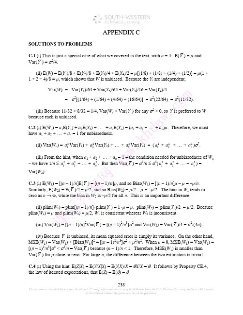
计量经济学导论:现代观点第四版习题答案DATA SET *****KIntroductory Econometrics: A Modern Approach, 4eJeffrey M. WooldridgeThis document contains a listing of all data sets that are provided with the fourth edition of Introductory Econometrics: A Modern Approach. For each data set, I list its source (wherever possible), where it is used or mentioned in the text (if it is), and, in some cases, notes on how an instructor might use the data set to generate new homework exercises, exam problems, or term projects. In some cases, I suggest ways to improve the data sets.Special thanks to Edmund Wooldridge, who provided valuable assistance in updating the page numbers for the fourth edition.401K.RAWSource: L.E. Papke (1995), “Participation in and Contributions to 401(k) Pension Plans: Evidence from Plan Data,” Journal of Human Resources 30, 311-325.Professor Papke kindly provided these data. She gathered them from the Internal Revenue Service’s Form 5500 tapes.Used in Text: pages 64, 80, 135-136, 173, 217, 685-686Notes: This data set is used in a variety of ways in the text. One additional possibility is to investigate whether the coefficients from the regression of prate on mrate, log(totemp) differ by whether the plan is a sole plan. The Chow test (see Section 7.4), and the less restrictive version that allows different intercepts, can be used.401KSUBS.RAWSource: A. Abadie (2003), “Semiparametric Instrumental VariableEstimation of Treatment Response Models,” Journal of Econometrics 113, 231-263.Professor Abadie kindly provided these data. He obtained them from the 1991 Survey of Income and Program Participation (SIPP).Used in Text: pages 165, 182, 222, 261, 279-280, 288, 298-299, 336, 542Notes: This data set can also be used to illustrate the binary response models, probit and logit, in Chapter 17, where, say, pira (an indicator for having an individual retirement account) is the dependent variable, and e401k [the 401(k) eligibility indicator] is the key explanatory variable.1*****.RAWSource: Data from the National Highway Traffic Safety Administration: “A Digest of State Alcohol-Highway Safety Related Legislation,” U.S. Department of Transportation, NHTSA. I used the third (1985), eighth (1990), and 13th (1995) editions.Used in Text: not usedNotes: This is not so much a data set as a summary of so-called “administrative per se” laws at the state level, for three different years. It could be supplemented with drunk-driving fatalities for a nice econometric analysis. In addition, the data for 2000 or later years can be added, forming the basis for a term project. Many other explanatory variables could be included. Unemployment rates, state-level tax rates on alcohol, and membership in MADD are just a few possibilities.*****.RAWSource: R.C. Fair (1978), “A Theory of Extramarital Affairs,” Journal of Political Economy 86, 45-61, 1978.I collected the data from Professor Fair’s web cite at the Yale University Department of Economics. He originally obtained the data from a survey by Psychology Today.Used in Text: not usedNotes: This is an interesting data set for problem sets, starting in Chapter 7. Even thoughnaffairs (number of extramarital affairs a woman reports) is a count variable, a linear model can be used as decent approximation. Or, you could ask the students to estimate a linear probability model for the binary indicator affair, equal to one of the woman reports having any extramarital affairs. One possibility is to test whether putting the single marriage rating variable, ratemarr, is enough, against the alternative that a full set of dummy variables is needed; see pages 237-238 for a similar example. This is also a good data set to illustrate Poisson regression (using naffairs) in Section 17.3 or probit and logit (using affair) in Section 17.1.*****.RAWSource: Jiyoung Kwon, a doctoral candidate in economics at MSU, kindly provided these data, which she obtained from the Domestic Airline Fares Consumer Report by the U.S. Department of Transportation.Used in Text: pages 501-502, 573Notes: This data set nicely illustrates the different estimates obtained when applying pooled OLS, random effects, and fixed effects.2APPLE.RAWSource: These data were used in the doctoral dissertation of Jeffrey Blend, Department of Agricultural Economics, Michigan State University, 1998. The thesis was supervised by Professor Eileen vanRavensway. Drs. Blend and van Ravensway kindly provided the data, which were obtained from a telephone survey conducted by the Institute for Public Policy and Social Research at MSU.Used in Text: pages 199, 222, 263, 618Notes: This data set is close to a true experimental data set because the price pairs facing afamily were randomly determined. In other words, the family head was presented with prices for the eco-labeled and regular apples, and then asked how much of each kind of apple they would buy at the given prices. As predicted by basic economics, the own price effect is strongly negative and the cross price effect is strongly positive. While the main dependent variable, ecolbs, piles up at zero, estimating a linear model is still worthwhile. Interestingly, because the survey design induces a strong positive correlation between the prices of eco-labeled and regular apples, there is an omitted variable problem if either of the price variables is dropped from the demand equation.A good exam question is to show a simple regression of ecolbs on ecoprc and then a multiple regression on both prices, and ask students to decide whether the price variables must be positively or negatively correlated.*****.RAWSources: Peterson's Guide to Four Year Colleges, 1994 and 1995 (24th and 25th editions). Princeton University Press. Princeton, NJ.The Official 1995 College Basketball Records Book, 1994, NCAA.1995 Information Please Sports Almanac (6th edition). Houghton Mifflin. New York, NY.Used in Text: page 690Notes: These data were collected by Patrick Tulloch, an MSU economics major, for a term project. The “athletic success” variablesare for the year prior to the enrollment and academic data. Updating these data to get a longer stretch of years, and including appearances in the “Sweet 16” NCAA basketball tournaments, would make for a more convincing analysis. With the growing popularity of women’s sports, especially basketball, an analysis that includes success in women’s athletics would be interesting.*****.RAWSources: Peterson's Guide to Four Year Colleges, 1995 (25th edition). Princeton University Press.1995 Information Please Sports Almanac (6th edition). Houghton Mifflin. New York, NYUsed in Text: page 6903Notes: These data were collected by Paul Anderson, an MSU economics major, for a term project. The score from football outcomes for natural rivals (Michigan-Michigan State, California-Stanford, Florida-Florida State, to name a few) is matched with application and academic data. The application and tuition data are for Fall 1994. Football records and scores are from 1993 football season. Extended these data to obtain a long stretch of panel data and other “natural” rivals could be very interesting.ATTEND.RAWSource: These data were collected by Professors Ronald Fisher and Carl Liedholm during a term in which they both taught principles of microeconomics at Michigan State University. Professors Fisher and Liedholm kindly gave me permission to use a random subset of their data, and their research assistant at the time, Jeffrey Guilfoyle, who completed his Ph.D. in economics at MSU, provided helpful hints.Used in Text: pages 111, 151, 198-199, 220-221Notes: The attendance figures were obtained by requiring students to slide their ID cards through a magnetic card reader, under the supervision of a teaching assistant. You might have the students use final, rather than the standardized variable, so that they can see the statistical significance of each variable remains exactly the same. The standardized variable is used only so that the coefficients measure effects in terms of standard deviations from the average score.AUDIT.RAWSource: These data come from a 1988 Urban Institute audit study in the Washington, D.C. area. I obtained them from the article “The Urban Institute Audit Studies: Their Methods andFindings,” by James J. Heckman and Peter Sieg elman. In Fix, M. and Struyk, R., eds., Clear and Convincing Evidence: Measurement of Discrimination in America. Washington, D.C.: Urban Institute Press, 1993, 187-258.Used in Text: pages 768-769, 776, 779BARIUM.RAWSource: C.M. Krupp and P.S. Pollard (1999), \Evidence from the U.S. Chemical Industry,\Canadian Journal of Economics 29, 199-227.Dr. Krupp kindly provided the data. They are monthly data covering February 1978 through December 1988.Used in Text: pages 357-358, 369, 373, 418, 422-423, 440, 655, 657, 665Note: Rather than just having intercept shifts for the different regimes, one could conduct a full Chow test across the different regimes.4BEAUTY.RAWSource: Hamermesh, D.S. and J.E. Biddle (1994), “Beauty and theLabor Market,” American Economic Review 84, 1174-1194.Professor Hamermesh kindly provided me with the data. For manageability, I have included only a subset of the variables, which results in somewhat larger sample sizes than reported for the regressions in the Hamermesh and Biddle paper.Used in Text: pages 236-237, 262-263BWGHT.RAWSource: J. Mullahy (1997), “Instrumental-Variable Estimation of Count Data Models:Applications to Models of Cigarette Smoking Behavior,” Review of Economics and Statistics 79, 596-593.Professor Mullahy kindly provided the data. He obtained them from the 1988 National Health Interview Survey.Used in Text: pages 18, 62, 110, 150-151, 164, 176, 182, 184-187, 255-256, 515-516BWGHT2.RAWSource: Dr. Zhehui Luo, a recent MSU Ph.D. in economics and Visiting Research Associate in the Department of Epidemiology at MSU, kindly provided these data. She obtained them from state files linking birth and infant death certificates, and from the National Center for Health Statistics natality and mortality data.Used in Text: pages 165, 211-222Notes: There are many possibilities with this data set. In addition to number of prenatal visits, smoking and alcohol consumption (during pregnancy) are included as explanatory variables. These can be added to equations of the kind found in Exercise C6.10. In addition, the one- and five-minute APGAR scores are included. These are measures of the well being of infants just after birth. An interesting feature of the score is that it is bounded between zero and 10, makinga linear model less than ideal. Still, a linear model would be informative, and you might ask students about predicted values less than zero or greater than 10.CAMPUS.RAWSource: These data were collected by Daniel Martin, a former MSU undergraduate, for a final project. They come from the FBI Uniform Crime Reports and are for the year 1992.Used in Text: pages 130-1315。
伍德里奇计量经济学导论第4版视频精讲!伍德里奇《计量经济学导论》(第4版)精讲班【教材精讲+考研真题串讲】来源:攻关学习网讲师:张冠甲/闫晶晶目录说明:本课程共包括42个高清视频(共54课时)。
序号名称1绪论2第1章计量经济学的性质与经济数据3第2章简单回归模型(1)4第2章简单回归模型(2)5第3章多元回归分析:估计(1)6第3章多元回归分析:估计(2)7第3章多元回归分析:估计(3)8第4章多元回归分析:推断(1)9第4章多元回归分析:推断(2)10第4章多元回归分析:推断(3)11第5章多元回归分析:OLS的渐进性(1)12第5章多元回归分析:OLS的渐进性(2)13第6章多元回归分析:深入专题(1)14第6章多元回归分析:深入专题(2)15第7章含有定性信息的多元回归分析:二值(或虚拟)变量(1)16第7章含有定性信息的多元回归分析:二值(或虚拟)变量(2)17第8章异方差性(1)18第8章异方差性(2)19第8章异方差性(3)20第8章异方差性(4)21第8章异方差性(5)22第9章模型设定和数据问题的深入探讨(1)23第9章模型设定和数据问题的深入探讨(2)24第9章模型设定和数据问题的深入探讨(3)25第9章模型设定和数据问题的深入探讨(4)26第9章模型设定和数据问题的深入探讨(5)27第10章时间序列数据的基本回归分析(1)28第10章时间序列数据的基本回归分析(2)29第11章OLS用于时间序列数据的其他问题(1)30第11章OLS用于时间序列数据的其他问题(2)31第12章时间序列回归中的序列相关和异方差(1)32第12章时间序列回归中的序列相关和异方差(2)33第13章跨时横截面的混合:简单面板数据方法(1)34第13章跨时横截面的混合:简单面板数据方法(2)35第14章高深的面板数据方法(1)36第14章高深的面板数据方法(2)37第15章工具变量估计与两阶段最小二乘法(1)38第15章工具变量估计与两阶段最小二乘法(2)39第16章联立方程模型40第17章限值因变量模型和样本选择纠正01:31:3241第18章时间序列高级专题42第19章一个经验项目的实施内容简介本课程是伍德里奇《计量经济学导论》(第4版)网授精讲班,为了帮助参加研究生招生考试指定考研参考书目为伍德里奇《计量经济学导论》(第4版)的考生复习专业课,我们根据教材和名校考研真题的命题规律精心讲解教材章节内容。
伍德里奇计量经济学导论摘要:一、伍德里奇《计量经济学导论》概述二、伍德里奇对计量经济学的定义与应用三、伍德里奇《计量经济学导论》的主要内容四、伍德里奇《计量经济学导论》的课后习题及其答案五、伍德里奇《计量经济学导论》的参考价值正文:一、伍德里奇《计量经济学导论》概述伍德里奇所著的《计量经济学导论》是一本广泛应用于经济学领域的经典教材,受到了全球范围内众多学者和学生的欢迎。
本书旨在介绍计量经济学的基本概念、方法和应用,帮助读者理解和掌握计量经济学的基本理论和实证分析技巧。
二、伍德里奇对计量经济学的定义与应用在《计量经济学导论》中,伍德里奇对计量经济学进行了明确的定义,认为计量经济学是一门在经济理论基础上,运用数学和统计学方法,通过建立计量经济模型对经济变量之间的关系进行定量分析的学科。
计量经济学的应用范围广泛,包括政策分析、市场预测、数据分析等诸多领域。
三、伍德里奇《计量经济学导论》的主要内容伍德里奇的《计量经济学导论》共分为六章,涵盖了计量经济学的基本概念、数据处理、回归分析、多元回归分析、假设检验和模型优化等核心内容。
具体来说,书中内容包括:1.计量经济学的性质与经济数据:介绍了计量经济学的基本概念,经济数据的来源和特点,以及如何利用经济数据进行计量分析。
2.简单回归模型:阐述了简单回归模型的基本原理,包括线性回归、最小二乘法、参数估计等。
3.多元回归分析:介绍了多元回归分析的基本概念,包括多元线性回归、多元逻辑回归等,以及如何进行多元回归模型的估计和检验。
4.假设检验:介绍了计量经济学中的假设检验原理,包括t 检验、F 检验等。
5.模型优化:探讨了如何优化计量经济模型,提高模型的预测能力和解释能力。
6.横截面数据的回归分析:介绍了横截面数据的回归分析方法,包括生产函数估计、需求函数估计等。
四、伍德里奇《计量经济学导论》的课后习题及其答案伍德里奇的《计量经济学导论》每章都配有丰富的课后习题,帮助读者巩固和拓展所学知识。