(完整版)六步学会用MATLAB做空间计量回归详细步骤
- 格式:doc
- 大小:415.79 KB
- 文档页数:22

matlab回归建模过程摘要:一、回归建模概述- 回归分析的定义- 回归建模的目的和意义二、MATLAB 回归建模过程- 一元线性回归- 数学模型定义- 模型参数估计- 检验、预测及控制- 多元线性回归- 数学模型定义- 模型参数估计- 多元线性回归中检验与预测- 逐步回归分析三、MATLAB 回归建模应用案例- 案例一:一元线性回归分析- 案例二:多元线性回归分析- 案例三:逐步回归分析正文:一、回归建模概述回归分析是一种研究变量之间关系的统计方法,通过建立一个数学模型,描述自变量与因变量之间的线性关系。
回归建模在实际应用中有着广泛的应用,如经济学、生物学、社会学等学科的研究中,可以帮助我们更好地理解变量之间的关系,并对未来趋势进行预测和控制。
MATLAB 是一种广泛应用于科学计算和数据分析的编程语言,提供了丰富的回归建模工具箱,可以帮助我们快速、高效地进行回归建模分析。
二、MATLAB 回归建模过程1.一元线性回归一元线性回归是最简单的回归分析方法,适用于只有一个自变量和一个因变量的情况。
在MATLAB 中,我们可以使用回归分析工具箱中的`regress`函数进行一元线性回归建模。
(1)数学模型定义一元线性回归的数学模型可以表示为:y = a + bx其中,y 表示因变量,x 表示自变量,a 和b 分别表示回归系数。
(2)模型参数估计在MATLAB 中,我们可以使用`regress`函数对模型参数进行估计。
函数的原型为:b = regress(y, x)其中,y 表示因变量向量,x 表示自变量向量,b 表示回归系数向量。
(3)检验、预测及控制在得到回归系数向量b 后,我们可以进行回归检验、预测以及控制。
2.多元线性回归多元线性回归适用于有多个自变量和因变量的情况。
在MATLAB 中,我们可以使用回归分析工具箱中的`polyfit`函数进行多元线性回归建模。
(1)数学模型定义多元线性回归的数学模型可以表示为:y = a0 + a1x1 + a2x2 + ...+ anxn其中,y 表示因变量,x1、x2、...、xn 表示自变量,a0、a1、a2、...、an 分别表示回归系数。

MATLAB回归分析工具箱使用方法1.数据准备在使用回归分析工具箱进行分析之前,首先需要准备好要使用的数据集。
数据集通常包含自变量和因变量,自变量是预测因变量的变量。
将数据集导入MATLAB中,并确保数据格式正确,可以使用MATLAB内置的导入工具或手动输入数据。
2.回归模型的选择在进行回归分析之前,需要选择适当的回归模型。
回归模型决定了如何拟合数据和生成预测。
常见的回归模型包括线性回归、多项式回归、逻辑回归等。
根据数据的特征和目的选择合适的回归模型。
3.拟合数据选择适当的回归模型后,可以使用回归分析工具箱中的函数来拟合数据。
常用的函数包括“fitlm”(线性回归)、“fitpoly”(多项式回归)、“fitglm”(逻辑回归)等。
将自变量和因变量传入对应的函数中,并得到拟合的模型。
例如,对于线性回归可以使用以下代码进行拟合:```mdl = fitlm(X,Y,'linear');```其中,X为自变量数据,Y为因变量数据,'linear'表示选择线性回归模型。
4.模型评估在拟合数据后,需要对模型进行评估以确定其拟合程度和预测性能。
可以使用回归分析工具箱中的函数来评估模型,如“plotResiduals”(绘制残差图)、“predict”(预测值)、“coefTest”(参数显著性检验)等。
通过观察残差图、计算R²值、进行参数显著性检验等方法,评估模型的拟合效果。
5.预测拟合好模型后,可以使用该模型进行预测未来的趋势。
使用“predict”函数可以生成预测值,并与实际值进行比较以评估模型的预测能力。
例如```Ypred = predict(mdl,Xnew);```其中,Xnew为新的自变量数据,Ypred为预测的因变量值。
6.结果可视化最后,可以使用MATLAB中的绘图工具来可视化回归分析的结果。
可以绘制拟合曲线、残差图、预测结果等,以便更直观地理解数据和模型。

matlab回归拟合回归拟合是一种常见的数据分析方法,通过建立数学模型来描述变量之间的关系,并利用已有数据对模型进行参数估计和预测。
Matlab是一种常用的数值计算软件,提供了丰富的工具和函数用于回归拟合。
本文将介绍使用Matlab进行回归拟合的基本步骤和常用函数。
一、数据导入与处理在进行回归拟合之前,首先需要将数据导入Matlab中,并进行必要的处理。
Matlab提供了多种导入数据的方式,如读取文本文件、导入Excel文件、数据库连接等。
例如,可以使用"readtable"函数读取文本文件数据,并将数据保存在一个表格变量中。
然后,可以使用表格变量的函数对数据进行预处理,如删除缺失值、选择有效变量等。
二、模型选择与建立回归拟合的目标是选择合适的数学模型来描述变量之间的关系。
在实际应用中,常用的回归模型包括线性回归、多项式回归、非线性回归等。
在Matlab中,可以使用"fitlm"函数进行线性回归拟合,使用"fitrgp"函数进行高斯过程回归拟合,使用"fitnlm"函数进行非线性最小二乘法拟合等。
这些函数提供了灵活的参数配置和模型选择功能,可以根据数据的特点选择合适的回归模型。
三、模型评估与诊断在进行回归拟合后,需要对拟合效果进行评估和诊断。
常用的评估指标包括均方误差(MSE)、决定系数(R-squared)、残差标准差等。
在Matlab中,可以使用"resubLoss"函数计算样本内误差,使用"coefTest"函数检验回归系数的显著性等。
此外,还可以通过绘制拟合曲线、残差图等进行可视化分析,以判断模型的合理性和拟合效果的好坏。
四、预测与应用完成回归拟合后,可以利用拟合模型进行预测和应用。
在Matlab中,可以使用"predict"函数对新的自变量进行预测,预测结果可以用于未知数据的预测、模型验证等。

利用MATLAB进行回归分析一、实验目的:1.了解回归分析的基本原理,掌握MATLAB实现的方法;2. 练习用回归分析解决实际问题。
二、实验内容:题目1社会学家认为犯罪与收入低、失业及人口规模有关,对20个城市的犯罪率y(每10万人中犯罪的人数)与年收入低于5000美元家庭的百分比1x、失业率2x和人口总数3x(千人)进行了调查,结果如下表。
(1)若1x~3x中至多只许选择2个变量,最好的模型是什么?(2)包含3个自变量的模型比上面的模型好吗?确定最终模型。
(3)对最终模型观察残差,有无异常点,若有,剔除后如何。
理论分析与程序设计:为了能够有一个较直观的认识,我们可以先分别作出犯罪率y与年收入低于5000美元家庭的百分比1x、失业率2x和人口总数x(千人)之间关系的散点图,根据大致分布粗略估计各因素造3成的影响大小,再通过逐步回归法确定应该选择哪几个自变量作为模型。
编写程序如下:clc;clear all;y=[11.2 13.4 40.7 5.3 24.8 12.7 20.9 35.7 8.7 9.6 14.5 26.9 15.736.2 18.1 28.9 14.9 25.8 21.7 25.7];%犯罪率(人/十万人)x1=[16.5 20.5 26.3 16.5 19.2 16.5 20.2 21.3 17.2 14.3 18.1 23.1 19.124.7 18.6 24.9 17.9 22.4 20.2 16.9];%低收入家庭百分比x2=[6.2 6.4 9.3 5.3 7.3 5.9 6.4 7.6 4.9 6.4 6.0 7.4 5.8 8.6 6.5 8.36.7 8.6 8.4 6.7];%失业率x3=[587 643 635 692 1248 643 1964 1531 713 749 7895 762 2793 741 625 854 716 921 595 3353];%总人口数(千人)figure(1),plot(x1,y,'*');figure(2),plot(x2,y,'*');figure(3),plot(x3,y,'*');X1=[x1',x2',x3'];stepwise(X1,y)运行结果与结论:犯罪率与低收入散点图犯罪率与失业率散点图犯罪率与人口总数散点图低收入与失业率作为自变量低收入与人口总数作为自变量失业率与人口总数作为自变量在图中可以明显看出前两图的线性程度很好,而第三个图的线性程度较差,从这个角度来说我们应该以失业率和低收入为自变量建立模型。

matlab回归建模过程摘要:一、引言二、MATLAB 回归建模的基本步骤1.数据的收集与整理2.建立回归模型3.模型参数估计4.模型检验5.模型预测与控制三、MATLAB 回归建模的实例分析1.一元线性回归2.多元线性回归3.逐步回归四、MATLAB 回归建模的优点与局限五、结论正文:一、引言MATLAB 是一种广泛应用于科学计算和工程设计的软件,其强大的数据处理和可视化功能为各种数学建模问题提供了便捷的解决方案。
在数学建模领域,回归分析是一种重要的方法,用于研究因变量和自变量之间的关系。
本文将详细介绍如何使用MATLAB 进行回归建模的过程。
二、MATLAB 回归建模的基本步骤1.数据的收集与整理在进行回归分析之前,首先需要收集相关的数据。
这些数据可以是实验测量值、历史统计数据等。
在收集到数据后,需要对其进行整理,将其转换为MATLAB 可以处理的格式。
2.建立回归模型在建立回归模型时,需要根据数据的特点和问题的实际背景选择合适的回归模型。
常见的回归模型有一元线性回归、多元线性回归、多项式回归、指数回归等。
3.模型参数估计在建立回归模型后,需要通过最小二乘法或其他方法对模型的参数进行估计。
MATLAB 提供了线性回归函数`regress`和多项式回归函数`polyfit`等工具用于模型参数的估计。
4.模型检验在模型参数估计完成后,需要对模型进行检验,以判断模型是否符合数据的实际情况。
常见的模型检验方法有残差分析、参数显著性检验等。
5.模型预测与控制在模型经过检验后,可以使用模型对未来的数据进行预测,或者利用模型对现有的数据进行控制。
MATLAB 提供了`predict`和`fit`等函数用于模型的预测和控制。
三、MATLAB 回归建模的实例分析1.一元线性回归以某市社会商品零售总额与职工工资总额的数据为例,可以使用一元线性回归模型进行建模。
首先输入数据,然后画出散点图,接着使用`regress`函数进行最小二乘回归,得到模型参数。
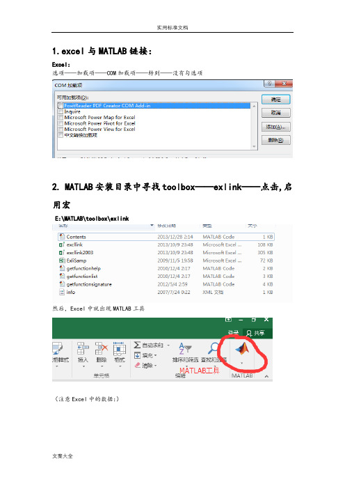
1.excel与MATLAB链接:Excel:选项——加载项——COM加载项——转到——没有勾选项2. MATLAB安装目录中寻找toolbox——exlink——点击,启用宏E:\MATLAB\toolbox\exlink然后,Excel中就出现MATLAB工具(注意Excel中的数据:)3.启动matlab(1)点击start MATLAB(2)senddata to matlab ,并对变量矩阵变量进行命名(注意:选取变量为数值,不包括各变量)(data表中数据进行命名)(空间权重进行命名)(3)导入MATLAB中的两个矩阵变量就可以看见4.将elhorst和jplv7两个程序文件夹复制到MATLAB安装目录的toolbox文件夹5.设置路径:6.输入程序,得出结果T=30;N=46;W=normw(W1);y=A(:,3);x=A(:,[4,6]);xconstant=ones(N*T,1); [nobs K]=size(x);results=ols(y,[xconstant x]);vnames=strvcat('logcit','intercept','logp','logy');prt_reg(results,vnames,1);sige=results.sige*((nobs-K)/nobs);loglikols=-nobs/2*log(2*pi*sige)-1/(2*sige)*results.resid'*results.resid% The (robust)LM tests developed by ElhorstLMsarsem_panel(results,W,y,[xconstant x]); % (Robust) LM tests解释每一行分别表示:附录:静态面板空间计量经济学一、OLS静态面板编程1、普通面板编程T=30;N=46;W=normw(W1);y=A(:,3);x=A(:,[4,6]);xconstant=ones(N*T,1);[nobs K]=size(x);results=ols(y,[xconstant x]);vnames=strvcat('logcit','intercept','logp','logy');prt_reg(results,vnames,1);sige=results.sige*((nobs-K)/nobs);loglikols=-nobs/2*log(2*pi*sige)-1/(2*sige)*results.resid'*results.resid% The (robust)LM tests developed by ElhorstLMsarsem_panel(results,W,y,[xconstant x]); % (Robust) LM tests2、空间固定OLS (spatial-fixed effects)T=30;N=46;W=normw(W1);y=A(:,3);x=A(:,[4,6]);xconstant=ones(N*T,1);[nobs K]=size(x);model=1;[ywith,xwith,meanny,meannx,meanty,meantx]=demean(y,x,N,T,mo del);results=ols(ywith,xwith);vnames=strvcat('logcit','logp','logy'); % should be changed if x is changedprt_reg(results,vnames);sfe=meanny-meannx*results.beta; % including the constant termyme = y - mean(y);et=ones(T,1);error=y-kron(et,sfe)-x*results.beta;rsqr1 = error'*error;rsqr2 = yme'*yme;FE_rsqr2 = 1.0 - rsqr1/rsqr2 % r-squared including fixed effectssige=results.sige*((nobs-K)/nobs);logliksfe=-nobs/2*log(2*pi*sige)-1/(2*sige)*results.resid'*results.residLMsarsem_panel(results,W,ywith,xwith); % (Robust) LM tests 3、时期固定OLS(time-period fixed effects)N=46;W=normw(W1);y=A(:,3);x=A(:,[4,6]);xconstant=ones(N*T,1);[nobs K]=size(x);model=2;[ywith,xwith,meanny,meannx,meanty,meantx]=demean(y,x,N,T,mo del);results=ols(ywith,xwith);vnames=strvcat('logcit','logp','logy'); % should be changed if x is changedprt_reg(results,vnames);tfe=meanty-meantx*results.beta; % including the constant termyme = y - mean(y);en=ones(N,1);error=y-kron(tfe,en)-x*results.beta;rsqr1 = error'*error;rsqr2 = yme'*yme;FE_rsqr2 = 1.0 - rsqr1/rsqr2 % r-squared including fixedsige=results.sige*((nobs-K)/nobs);logliktfe=-nobs/2*log(2*pi*sige)-1/(2*sige)*results.resid'*results.residLMsarsem_panel(results,W,ywith,xwith); % (Robust) LM tests4、空间与时间双固定模型T=30;N=46;W=normw(W1);y=A(:,3);x=A(:,[4,6]);xconstant=ones(N*T,1);[nobs K]=size(x);model=3;[ywith,xwith,meanny,meannx,meanty,meantx]=demean(y,x,N,T,mo del);results=ols(ywith,xwith);vnames=strvcat('logcit','logp','logy'); % should be changed if x is changedprt_reg(results,vnames)en=ones(N,1);et=ones(T,1);intercept=mean(y)-mean(x)*results.beta;sfe=meanny-meannx*results.beta-kron(en,intercept);tfe=meanty-meantx*results.beta-kron(et,intercept);yme = y - mean(y);ent=ones(N*T,1);error=y-kron(tfe,en)-kron(et,sfe)-x*results.beta-kron(ent,intercept);rsqr1 = error'*error;rsqr2 = yme'*yme;FE_rsqr2 = 1.0 - rsqr1/rsqr2 % r-squared including fixed effectssige=results.sige*((nobs-K)/nobs);loglikstfe=-nobs/2*log(2*pi*sige)-1/(2*sige)*results.resid'*results.residLMsarsem_panel(results,W,ywith,xwith); % (Robust) LM tests二、静态面板SAR模型1、无固定效应(No fixed effects)T=30;N=46;W=normw(W1);y=A(:,[3]);x=A(:,[4,6]);for t=1:Tt1=(t-1)*N+1;t2=t*N;wx(t1:t2,:)=W*x(t1:t2,:);endxconstant=ones(N*T,1);[nobs K]=size(x);info.lflag=0;info.model=0;info.fe=0;results=sar_panel_FE(y,[xconstant x],W,T,info);vnames=strvcat('logcit','intercept','logp','logy');prt_spnew(results,vnames,1)% Print out effects estimatesspat_model=0;direct_indirect_effects_estimates(results,W,spat_model); panel_effects_sar(results,vnames,W);2、空间固定效应(Spatial fixed effects)T=30;N=46;W=normw(W1);y=A(:,[3]);x=A(:,[4,6]);for t=1:Tt1=(t-1)*N+1;t2=t*N;wx(t1:t2,:)=W*x(t1:t2,:);endxconstant=ones(N*T,1);[nobs K]=size(x);info.lflag=0;info.model=1;info.fe=0;results=sar_panel_FE(y,x,W,T,info);vnames=strvcat('logcit','logp','logy');prt_spnew(results,vnames,1)% Print out effects estimatesspat_model=0;direct_indirect_effects_estimates(results,W,spat_model); panel_effects_sar(results,vnames,W);3、时点固定效应(Time period fixed effects)T=30;N=46;W=normw(W1);y=A(:,[3]);x=A(:,[4,6]);for t=1:Tt1=(t-1)*N+1;t2=t*N;wx(t1:t2,:)=W*x(t1:t2,:);endxconstant=ones(N*T,1);[nobs K]=size(x);info.lflag=0; % required for exact resultsinfo.model=2;info.fe=0; % Do not print intercept and fixed effects; use info.fe=1 to turn on results=sar_panel_FE(y,x,W,T,info);vnames=strvcat('logcit','logp','logy');prt_spnew(results,vnames,1)% Print out effects estimatesspat_model=0;direct_indirect_effects_estimates(results,W,spat_model);panel_effects_sar(results,vnames,W);4、双固定效应(Spatial and time period fixed effects)T=30;N=46;W=normw(W1);y=A(:,[3]);x=A(:,[4,6]);for t=1:Tt1=(t-1)*N+1;t2=t*N;wx(t1:t2,:)=W*x(t1:t2,:);endxconstant=ones(N*T,1);[nobs K]=size(x);info.lflag=0; % required for exact resultsinfo.model=3;info.fe=0; % Do not print intercept and fixed effects; use info.fe=1 to turn on results=sar_panel_FE(y,x,W,T,info);vnames=strvcat('logcit','logp','logy');prt_spnew(results,vnames,1)% Print out effects estimatesspat_model=0;direct_indirect_effects_estimates(results,W,spat_model);panel_effects_sar(results,vnames,W);三、静态面板SDM模型1、无固定效应(No fixed effects)T=30;N=46;W=normw(W1);y=A(:,[3]);x=A(:,[4,6]);for t=1:Tt1=(t-1)*N+1;t2=t*N;wx(t1:t2,:)=W*x(t1:t2,:);endxconstant=ones(N*T,1);[nobs K]=size(x);info.lflag=0;info.model=0;info.fe=0;results=sar_panel_FE(y,[xconstant x wx],W,T,info);vnames=strvcat('logcit','intercept','logp','logy','W*logp','W*logy');prt_spnew(results,vnames,1)% Print out effects estimatesspat_model=1;direct_indirect_effects_estimates(results,W,spat_model);panel_effects_sdm(results,vnames,W);2、空间固定效应(Spatial fixed effects)T=30;N=46;W=normw(W1);y=A(:,[3]);x=A(:,[4,6]);for t=1:Tt1=(t-1)*N+1;t2=t*N;wx(t1:t2,:)=W*x(t1:t2,:);endxconstant=ones(N*T,1);[nobs K]=size(x);info.lflag=0; % required for exact resultsinfo.model=1;info.fe=0; % Do not print intercept and fixed effects; use info.fe=1 to turn on results=sar_panel_FE(y,[x wx],W,T,info);vnames=strvcat('logcit','logp','logy','W*logp','W*logy');prt_spnew(results,vnames,1)% Print out effects estimatesspat_model=1;direct_indirect_effects_estimates(results,W,spat_model);panel_effects_sdm(results,vnames,W);3、时点固定效应(Time period fixed effects)T=30;N=46;W=normw(W1);y=A(:,[3]);x=A(:,[4,6]);for t=1:Tt1=(t-1)*N+1;t2=t*N;wx(t1:t2,:)=W*x(t1:t2,:);endxconstant=ones(N*T,1);[nobs K]=size(x);info.lflag=0; % required for exact resultsinfo.model=2;info.fe=0; % Do not print intercept and fixed effects; use info.fe=1 to turn on % New routines to calculate effects estimatesresults=sar_panel_FE(y,[x wx],W,T,info);vnames=strvcat('logcit','logp','logy','W*logp','W*logy');% Print out coefficient estimatesprt_spnew(results,vnames,1)% Print out effects estimatesspat_model=1;direct_indirect_effects_estimates(results,W,spat_model);panel_effects_sdm(results,vnames,W)4、双固定效应(Spatial and time period fixed effects)T=30;N=46;W=normw(W1);y=A(:,[3]);x=A(:,[4,6]);for t=1:Tt1=(t-1)*N+1;t2=t*N;wx(t1:t2,:)=W*x(t1:t2,:);endxconstant=ones(N*T,1);[nobs K]=size(x);info.bc=0;info.lflag=0; % required for exact resultsinfo.model=3;info.fe=0; % Do not print intercept and fixed effects; use info.fe=1 to turn on results=sar_panel_FE(y,[x wx],W,T,info);vnames=strvcat('logcit','logp','logy','W*logp','W*logy');prt_spnew(results,vnames,1)% Print out effects estimatesspat_model=1;direct_indirect_effects_estimates(results,W,spat_model);panel_effects_sdm(results,vnames,W)wald test spatial lag% Wald test for spatial Durbin model against spatial lag modelbtemp=results.parm;varcov=results.cov;Rafg=zeros(K,2*K+2);for k=1:KRafg(k,K+k)=1; % R(1,3)=0 and R(2,4)=0;endWald_spatial_lag=(Rafg*btemp)'*inv(Rafg*varcov*Rafg')*Rafg*btempprob_spatial_lag=1-chis_cdf (Wald_spatial_lag, K)wald test spatial error% Wald test spatial Durbin model against spatial error modelR=zeros(K,1);for k=1:KR(k)=btemp(2*K+1)*btemp(k)+btemp(K+k); % k changed in 1, 7/12/2010% R(1)=btemp(5)*btemp(1)+btemp(3);% R(2)=btemp(5)*btemp(2)+btemp(4);endRafg=zeros(K,2*K+2);for k=1:KRafg(k,k) =btemp(2*K+1); % k changed in 1, 7/12/2010Rafg(k,K+k) =1;Rafg(k,2*K+1)=btemp(k);% Rafg(1,1)=btemp(5);Rafg(1,3)=1;Rafg(1,5)=btemp(1);% Rafg(2,2)=btemp(5);Rafg(2,4)=1;Rafg(2,5)=btemp(2);endWald_spatial_error=R'*inv(Rafg*varcov*Rafg')*Rprob_spatial_error=1-chis_cdf (Wald_spatial_error,K)LR test spatial lagresultssar=sar_panel_FE(y,x,W,T,info);LR_spatial_lag=-2*(resultssar.lik-results.lik)prob_spatial_lag=1-chis_cdf (LR_spatial_lag,K)LR test spatial errorresultssem=sem_panel_FE(y,x,W,T,info);LR_spatial_error=-2*(resultssem.lik-results.lik)prob_spatial_error=1-chis_cdf (LR_spatial_error,K)5、空间随机效应与时点固定效应模型T=30;N=46;W=normw(W1);y=A(:,[3]);x=A(:,[4,6]);for t=1:Tt1=(t-1)*N+1;t2=t*N;wx(t1:t2,:)=W*x(t1:t2,:);endxconstant=ones(N*T,1);[nobs K]=size(x);[ywith,xwith,meanny,meannx,meanty,meantx]=demean(y,[x wx],N,T,2); % 2=time dummies info.model=1;results=sar_panel_RE(ywith,xwith,W,T,info);prt_spnew(results,vnames,1)spat_model=1;direct_indirect_effects_estimates(results,W,spat_model);panel_effects_sdm(results,vnames,W)wald test spatial lagbtemp=results.parm(1:2*K+2);varcov=results.cov(1:2*K+2,1:2*K+2);Rafg=zeros(K,2*K+2);for k=1:KRafg(k,K+k)=1; % R(1,3)=0 and R(2,4)=0;endWald_spatial_lag=(Rafg*btemp)'*inv(Rafg*varcov*Rafg')*Rafg*btempprob_spatial_lag= 1-chis_cdf (Wald_spatial_lag, K)wald test spatial errorR=zeros(K,1);for k=1:KR(k)=btemp(2*K+1)*btemp(k)+btemp(K+k); % k changed in 1, 7/12/2010 % R(1)=btemp(5)*btemp(1)+btemp(3);% R(2)=btemp(5)*btemp(2)+btemp(4);endRafg=zeros(K,2*K+2);for k=1:KRafg(k,k) =btemp(2*K+1); % k changed in 1, 7/12/2010Rafg(k,K+k) =1;Rafg(k,2*K+1)=btemp(k);% Rafg(1,1)=btemp(5);Rafg(1,3)=1;Rafg(1,5)=btemp(1);% Rafg(2,2)=btemp(5);Rafg(2,4)=1;Rafg(2,5)=btemp(2);endWald_spatial_error=R'*inv(Rafg*varcov*Rafg')*Rprob_spatial_error= 1-chis_cdf (Wald_spatial_error,K)LR test spatial lagresultssar=sar_panel_RE(ywith,xwith(:,1:K),W,T,info);LR_spatial_lag=-2*(resultssar.lik-results.lik)prob_spatial_lag=1-chis_cdf (LR_spatial_lag,K)LR test spatial errorresultssem=sem_panel_RE(ywith,xwith(:,1:K),W,T,info);LR_spatial_error=-2*(resultssem.lik-results.lik)prob_spatial_error=1-chis_cdf (LR_spatial_error,K)四、静态面板SEM模型1、无固定效应(No fixed effects)T=30;W=normw(W1);y=A(:,[3]);x=A(:,[4,6]);for t=1:Tt1=(t-1)*N+1;t2=t*N;wx(t1:t2,:)=W*x(t1:t2,:);endxconstant=ones(N*T,1);[nobs K]=size(x);info.lflag=0;info.model=0;info.fe=0;results=sem_panel_FE(y,[xconstant x],W,T,info);vnames=strvcat('logcit','intercept','logp','logy');prt_spnew(results,vnames,1)% Print out effects estimatesspat_model=0;direct_indirect_effects_estimates(results,W,spat_model); panel_effects_sar(results,vnames,W);2、空间固定效应(Spatial fixed effects)T=30;N=46;W=normw(W1);y=A(:,[3]);x=A(:,[4,6]);for t=1:Tt1=(t-1)*N+1;t2=t*N;wx(t1:t2,:)=W*x(t1:t2,:);endxconstant=ones(N*T,1);[nobs K]=size(x);info.lflag=0;info.model=1;info.fe=0;results=sem_panel_FE(y,x,W,T,info);vnames=strvcat('logcit','logp','logy');prt_spnew(results,vnames,1)% Print out effects estimatesspat_model=0;direct_indirect_effects_estimates(results,W,spat_model); panel_effects_sar(results,vnames,W);3、时点固定效应(Time period fixed effects)N=46;W=normw(W1);y=A(:,[3]);x=A(:,[4,6]);for t=1:Tt1=(t-1)*N+1;t2=t*N;wx(t1:t2,:)=W*x(t1:t2,:);endxconstant=ones(N*T,1);[nobs K]=size(x);info.lflag=0; % required for exact resultsinfo.model=2;info.fe=0; % Do not print intercept and fixed effects; use info.fe=1 to turn on results=sem_panel_FE(y,x,W,T,info);vnames=strvcat('logcit','logp','logy');prt_spnew(results,vnames,1)% Print out effects estimatesspat_model=0;direct_indirect_effects_estimates(results,W,spat_model);panel_effects_sar(results,vnames,W);4、双固定效应(Spatial and time period fixed effects)T=30;N=46;W=normw(W1);y=A(:,[3]);x=A(:,[4,6]);for t=1:Tt1=(t-1)*N+1;t2=t*N;wx(t1:t2,:)=W*x(t1:t2,:);endxconstant=ones(N*T,1);[nobs K]=size(x);info.lflag=0; % required for exact resultsinfo.model=3;info.fe=0; % Do not print intercept and fixed effects; use info.fe=1 to turn on results=sem_panel_FE(y,x,W,T,info);vnames=strvcat('logcit','logp','logy');prt_spnew(results,vnames,1)% Print out effects estimatesspat_model=0;direct_indirect_effects_estimates(results,W,spat_model);panel_effects_sar(results,vnames,W);五、静态面板SDEM模型1、无固定效应(No fixed effects)T=30;N=46;W=normw(W1);y=A(:,[3]);x=A(:,[4,6]);for t=1:Tt1=(t-1)*N+1;t2=t*N;wx(t1:t2,:)=W*x(t1:t2,:);endxconstant=ones(N*T,1);[nobs K]=size(x);info.lflag=0;info.model=0;info.fe=0;results=sem_panel_FE(y,[xconstant x wx],W,T,info);vnames=strvcat('logcit','intercept','logp','logy','W*logp','W*logy');prt_spnew(results,vnames,1)% Print out effects estimatesspat_model=1;direct_indirect_effects_estimates(results,W,spat_model);panel_effects_sdm(results,vnames,W);2、空间固定效应(Spatial fixed effects)T=30;N=46;W=normw(W1);y=A(:,[3]);x=A(:,[4,6]);for t=1:Tt1=(t-1)*N+1;t2=t*N;wx(t1:t2,:)=W*x(t1:t2,:);endxconstant=ones(N*T,1);[nobs K]=size(x);info.lflag=0; % required for exact resultsinfo.model=1;info.fe=0; % Do not print intercept and fixed effects; use info.fe=1 to turn on results=sem_panel_FE(y,[x wx],W,T,info);vnames=strvcat('logcit','logp','logy','W*logp','W*logy');prt_spnew(results,vnames,1)% Print out effects estimatesspat_model=1;direct_indirect_effects_estimates(results,W,spat_model);panel_effects_sdm(results,vnames,W);3、时点固定效应(Time period fixed effects)T=30;N=46;W=normw(W1);y=A(:,[3]);x=A(:,[4,6]);for t=1:Tt1=(t-1)*N+1;t2=t*N;wx(t1:t2,:)=W*x(t1:t2,:);endxconstant=ones(N*T,1);[nobs K]=size(x);info.lflag=0; % required for exact resultsinfo.model=2;info.fe=0; % Do not print intercept and fixed effects; use info.fe=1 to turn on % New routines to calculate effects estimatesresults=sem_panel_FE(y,[x wx],W,T,info);vnames=strvcat('logcit','logp','logy','W*logp','W*logy');% Print out coefficient estimatesprt_spnew(results,vnames,1)% Print out effects estimatesspat_model=1;direct_indirect_effects_estimates(results,W,spat_model);panel_effects_sdm(results,vnames,W)4、双固定效应(Spatial and time period fixed effects)T=30;N=46;W=normw(W1);y=A(:,[3]);x=A(:,[4,6]);for t=1:Tt1=(t-1)*N+1;t2=t*N;wx(t1:t2,:)=W*x(t1:t2,:);endxconstant=ones(N*T,1);[nobs K]=size(x);info.bc=0;info.lflag=0; % required for exact resultsinfo.model=3;info.fe=0; % Do not print intercept and fixed effects; use info.fe=1 to turn on results=sem_panel_FE(y,[x wx],W,T,info);vnames=strvcat('logcit','logp','logy','W*logp','W*logy');prt_spnew(results,vnames,1)% Print out effects estimatesspat_model=1;direct_indirect_effects_estimates(results,W,spat_model);panel_effects_sdm(results,vnames,W)。
Matlab中的回归分析技术实践引言回归分析是统计学中常用的一种分析方法,用于研究因变量和一个或多个自变量之间的关系。
Matlab是一种强大的数值计算软件,具有丰富的统计分析工具和函数。
通过Matlab中的回归分析技术,我们可以深入理解数据背后的规律,并预测未来的趋势。
本文将介绍Matlab中常用的回归分析方法和技巧,并通过实例演示其实践应用。
一、简单线性回归分析简单线性回归是回归分析的最基本形式,用于研究一个自变量和一个因变量之间的线性关系。
在Matlab中,可以使用`fitlm`函数进行简单线性回归分析。
以下是一个示例代码:```Matlabx = [1, 2, 3, 4, 5]';y = [2, 4, 6, 8, 10]';lm = fitlm(x, y);```这段代码中,我们定义了两个向量x和y作为自变量和因变量的观测值。
使用`fitlm`函数可以得到一个线性回归模型lm。
通过这个模型,我们可以获取回归系数、拟合优度、显著性检验等信息。
二、多元线性回归分析多元线性回归分析允许我们研究多个自变量与一个因变量的关系。
在Matlab中,可以使用`fitlm`函数进行多元线性回归分析。
以下是一个示例代码:```Matlabx1 = [1, 2, 3, 4, 5]';x2 = [0, 1, 0, 1, 0]';y = [2, 4, 6, 8, 10]';X = [ones(size(x1)), x1, x2];lm = fitlm(X, y);```这段代码中,我们定义了两个自变量x1和x2,以及一个因变量y的观测值。
通过将常数项和自变量组合成一个设计矩阵X,使用`fitlm`函数可以得到一个多元线性回归模型lm。
通过这个模型,我们可以获取回归系数、拟合优度、显著性检验等信息。
三、非线性回归分析在实际问题中,很多情况下变量之间的关系并不是线性的。
非线性回归分析可以更准确地建模非线性关系。
如何在MATLAB中进行统计回归分析统计回归分析是一种被广泛应用于数据科学和统计学领域的技术。
它被用来分析变量之间的关系,并预测一个或多个自变量对因变量的影响。
在MATLAB中,有许多强大的工具和函数可以帮助我们进行统计回归分析。
本文将讨论如何在MATLAB中使用这些功能进行统计回归分析。
1. 数据导入与预处理在进行回归分析之前,首先需要将数据导入到MATLAB中。
MATLAB支持多种数据格式,如CSV、Excel、文本文件等。
可以使用readmatrix或readtable等函数读取数据,根据数据的特点选择合适的函数。
在导入数据之后,通常需要对数据进行预处理。
这包括处理缺失值、异常值以及数据的标准化。
MATLAB提供了一系列函数来处理这些问题,如isnan、isoutlier和zscore等。
2. 单变量回归分析单变量回归分析是最基本的回归分析方法。
它用于分析一个自变量对一个因变量的影响。
在MATLAB中,可以使用fitlm函数进行单变量回归分析。
fitlm函数需要输入自变量和因变量的数据,然后可以对回归模型进行拟合,并得到回归系数、残差等统计信息。
使用plot函数可以绘制回归模型的拟合曲线,以及残差的散点图。
通过观察残差的分布,可以评估拟合模型的合理性。
3. 多变量回归分析多变量回归分析是在一个或多个自变量对一个因变量的影响进行分析。
在MATLAB中,可以使用fitlm函数或者fitlmulti函数实现多变量回归分析。
fitlm函数可以处理多个自变量,但是需要手动选择自变量,并提供自变量和因变量的数据。
fitlmulti函数则可以自动选择最佳的自变量组合,并进行回归拟合。
它需要提供自变量和因变量的数据矩阵。
多变量回归分析的结果可以通过查看回归系数和残差来解释。
还可以使用plot函数绘制回归模型的拟合曲面或曲线,以便更好地理解自变量对因变量的影响。
4. 方差分析方差分析是一种常用的统计方法,用于比较两个或多个因素对因变量的影响。
MATLAB回归分析工具箱使用方法下面将详细介绍如何使用MATLAB中的回归分析工具箱进行回归分析。
1.数据准备回归分析需要一组自变量和一个因变量。
首先,你需要将数据准备好,并确保自变量和因变量是数值型数据。
你可以将数据存储在MATLAB工作区中的变量中,也可以从外部文件中读取数据。
2.导入回归分析工具箱在MATLAB命令窗口中输入"regstats"命令来导入回归分析工具箱。
这将使得回归分析工具箱中的函数和工具可用于你的分析。
3.线性回归分析线性回归分析是回归分析的最基本形式。
你可以使用"regstats"函数进行线性回归分析。
以下是一个简单的例子:```matlabdata = load('data.mat'); % 从外部文件加载数据X = data.X; % 自变量y = data.y; % 因变量stats = regstats(y, X); % 执行线性回归分析beta = stats.beta; % 提取回归系数rsquare = stats.rsquare; % 提取判定系数R^2```在上面的例子中,"regstats"函数将自变量X和因变量y作为参数,并返回一个包含回归系数beta和判定系数R^2的结构体stats。
4.非线性回归分析如果你的数据不适合线性回归模型,你可以尝试非线性回归分析。
回归分析工具箱提供了用于非线性回归分析的函数,如"nonlinearmodel.fit"。
以下是一个非线性回归分析的例子:```matlabx=[0.10.20.5125]';%自变量y=[0.92.22.83.66.58.9]';%因变量f = fittype('a*exp(b*x)'); % 定义非线性模型model = fit(x, y, f); % 执行非线性回归分析coeffs = model.coefficients; % 提取模型系数```在上面的例子中,"fittype"函数定义了一个指数型的非线性模型,并且"fit"函数将自变量x和因变量y与该模型拟合,返回包含模型系数的结构体model。
利用 Matlab 作回归分析一元线性回归模型:2,(0,)y x N αβεεσ=++求得经验回归方程:ˆˆˆyx αβ=+ 统计量: 总偏差平方和:21()n i i SST y y ==-∑,其自由度为1T f n =-; 回归平方和:21ˆ()n i i SSR y y ==-∑,其自由度为1R f =; 残差平方和:21ˆ()n i i i SSE y y ==-∑,其自由度为2E f n =-;它们之间有关系:SST=SSR+SSE 。
一元回归分析的相关数学理论可以参见《概率论与数理统计教程》,下面仅以示例说明如何利用Matlab 作回归分析。
【例1】为了了解百货商店销售额x 与流通费率(反映商业活动的一个质量指标,指每元商品流转额所分摊的流通费用)y 之间的关系,收集了九个商店的有关数据,见下表1.试建立流通费率y 与销售额x 的回归方程。
表1 销售额与流通费率数据【分析】:首先绘制散点图以直观地选择拟合曲线,这项工作可结合相关专业领域的知识和经验进行,有时可能需要多种尝试。
选定目标函数后进行线性化变换,针对变换后的线性目标函数进行回归建模与评价,然后还原为非线性回归方程。
【Matlab数据处理】:【Step1】:绘制散点图以直观地选择拟合曲线x=[1.5 4.5 7.5 10.5 13.5 16.5 19.5 22.5 25.5];y=[7.0 4.8 3.6 3.1 2.7 2.5 2.4 2.3 2.2];plot(x,y,'-o')输出图形见图1。
510152025图1 销售额与流通费率数据散点图根据图1,初步判断应以幂函数曲线为拟合目标,即选择非线性回归模型,目标函数为:(0)b y ax b =< 其线性化变换公式为:ln ,ln v y u x == 线性函数为:ln v a bu =+【Step2】:线性化变换即线性回归建模(若选择为非线性模型)与模型评价% 线性化变换u=log(x)';v=log(y)';% 构造资本论观测值矩阵mu=[ones(length(u),1) u];alpha=0.05;% 线性回归计算[b,bint,r,rint,states]=regress(v,mu,alpha)输出结果:b =[ 2.1421; -0.4259]表示线性回归模型ln=+中:lna=2.1421,b=-0.4259;v a bu即拟合的线性回归模型为=-;y x2.14210.4259bint =[ 2.0614 2.2228; -0.4583 -0.3934]表示拟合系数lna和b的100(1-alpha)%的置信区间分别为:[2.0614 2.2228]和[-0.4583 -0.3934];r =[ -0.0235 0.0671 -0.0030 -0.0093 -0.0404 -0.0319 -0.0016 0.0168 0.0257]表示模型拟合残差向量;rint =[ -0.0700 0.02300.0202 0.1140-0.0873 0.0813-0.0939 0.0754-0.1154 0.0347-0.1095 0.0457-0.0837 0.0805-0.0621 0.0958-0.0493 0.1007]表示模型拟合残差的100(1-alpha)%的置信区间;states =[0.9928 963.5572 0.0000 0.0012] 表示包含20.9928SSR R SST==、 方差分析的F 统计量/963.5572//(2)R E SSR f SSR F SSE f SSE n ===-、 方差分析的显著性概率((1,2))0p P F n F =->≈; 模型方差的估计值2ˆ0.00122SSE n σ==-。
1.excel与MATLAB链接:Excel:选项——加载项——COM加载项——转到——没有勾选项2. MATLAB安装目录中寻找toolbox——exlink——点击,启用宏E:\MATLAB\toolbox\exlink然后,Excel中就出现MATLAB工具(注意Excel中的数据:)3.启动matlab(1)点击start MATLAB(2)senddata to matlab ,并对变量矩阵变量进行命名(注意:选取变量为数值,不包括各变量)(data表中数据进行命名)(空间权重进行命名)(3)导入MATLAB中的两个矩阵变量就可以看见4.将elhorst和jplv7两个程序文件夹复制到MATLAB安装目录的toolbox文件夹5.设置路径:6.输入程序,得出结果T=30;N=46;W=normw(W1);y=A(:,3);x=A(:,[4,6]);xconstant=ones(N*T,1); [nobs K]=size(x);results=ols(y,[xconstant x]);vnames=strvcat('logcit','intercept','logp','logy');prt_reg(results,vnames,1);sige=results.sige*((nobs-K)/nobs);loglikols=-nobs/2*log(2*pi*sige)-1/(2*sige)*results.resid'*results.resid % The (robust)LM tests developed by ElhorstLMsarsem_panel(results,W,y,[xconstant x]); % (Robust) LM tests 解释附录:静态面板空间计量经济学一、OLS静态面板编程1、普通面板编程T=30;N=46;W=normw(W1);y=A(:,3);x=A(:,[4,6]);xconstant=ones(N*T,1);[nobs K]=size(x);results=ols(y,[xconstant x]);vnames=strvcat('logcit','intercept','logp','logy');prt_reg(results,vnames,1);sige=results.sige*((nobs-K)/nobs);loglikols=-nobs/2*log(2*pi*sige)-1/(2*sige)*results.resid'*results.resid % The (robust)LM tests developed by ElhorstLMsarsem_panel(results,W,y,[xconstant x]); % (Robust) LM tests2、空间固定OLS (spatial-fixed effects)T=30;N=46;W=normw(W1);y=A(:,3);x=A(:,[4,6]);xconstant=ones(N*T,1);[nobs K]=size(x);model=1;[ywith,xwith,meanny,meannx,meanty,meantx]=demean(y,x,N,T,model );results=ols(ywith,xwith);vnames=strvcat('logcit','logp','logy'); % should be changed if x is changedprt_reg(results,vnames);sfe=meanny-meannx*results.beta; % including the constant term yme = y - mean(y);et=ones(T,1);error=y-kron(et,sfe)-x*results.beta;rsqr1 = error'*error;rsqr2 = yme'*yme;FE_rsqr2 = 1.0 - rsqr1/rsqr2 % r-squared including fixed effectssige=results.sige*((nobs-K)/nobs);logliksfe=-nobs/2*log(2*pi*sige)-1/(2*sige)*results.resid'*results.resid LMsarsem_panel(results,W,ywith,xwith); % (Robust) LM tests3、时期固定OLS(time-period fixed effects)T=30;N=46;W=normw(W1);y=A(:,3);x=A(:,[4,6]);xconstant=ones(N*T,1);[nobs K]=size(x);model=2;[ywith,xwith,meanny,meannx,meanty,meantx]=demean(y,x,N,T,model );results=ols(ywith,xwith);vnames=strvcat('logcit','logp','logy'); % should be changed if x is changedprt_reg(results,vnames);tfe=meanty-meantx*results.beta; % including the constant termyme = y - mean(y);en=ones(N,1);error=y-kron(tfe,en)-x*results.beta;rsqr1 = error'*error;rsqr2 = yme'*yme;FE_rsqr2 = 1.0 - rsqr1/rsqr2 % r-squared including fixed effectssige=results.sige*((nobs-K)/nobs);logliktfe=-nobs/2*log(2*pi*sige)-1/(2*sige)*results.resid'*results.resid LMsarsem_panel(results,W,ywith,xwith); % (Robust) LM tests4、空间与时间双固定模型T=30;N=46;W=normw(W1);y=A(:,3);x=A(:,[4,6]);xconstant=ones(N*T,1);[nobs K]=size(x);model=3;[ywith,xwith,meanny,meannx,meanty,meantx]=demean(y,x,N,T,model );results=ols(ywith,xwith);vnames=strvcat('logcit','logp','logy'); % should be changed if x is changedprt_reg(results,vnames)en=ones(N,1);et=ones(T,1);intercept=mean(y)-mean(x)*results.beta;sfe=meanny-meannx*results.beta-kron(en,intercept);tfe=meanty-meantx*results.beta-kron(et,intercept);yme = y - mean(y);ent=ones(N*T,1);error=y-kron(tfe,en)-kron(et,sfe)-x*results.beta-kron(ent,intercept); rsqr1 = error'*error;rsqr2 = yme'*yme;FE_rsqr2 = 1.0 - rsqr1/rsqr2 % r-squared including fixed effectssige=results.sige*((nobs-K)/nobs);loglikstfe=-nobs/2*log(2*pi*sige)-1/(2*sige)*results.resid'*results.residLMsarsem_panel(results,W,ywith,xwith); % (Robust) LM tests二、静态面板SAR模型1、无固定效应(No fixed effects)T=30;N=46;W=normw(W1);y=A(:,[3]);x=A(:,[4,6]);for t=1:Tt1=(t-1)*N+1;t2=t*N;wx(t1:t2,:)=W*x(t1:t2,:);endxconstant=ones(N*T,1);[nobs K]=size(x);info.lflag=0;info.model=0;info.fe=0;results=sar_panel_FE(y,[xconstant x],W,T,info);vnames=strvcat('logcit','intercept','logp','logy');prt_spnew(results,vnames,1)% Print out effects estimatesspat_model=0;direct_indirect_effects_estimates(results,W,spat_model); panel_effects_sar(results,vnames,W);2、空间固定效应(Spatial fixed effects)T=30;N=46;W=normw(W1);y=A(:,[3]);x=A(:,[4,6]);for t=1:Tt1=(t-1)*N+1;t2=t*N;wx(t1:t2,:)=W*x(t1:t2,:);endxconstant=ones(N*T,1);[nobs K]=size(x);info.lflag=0;info.model=1;info.fe=0;results=sar_panel_FE(y,x,W,T,info);vnames=strvcat('logcit','logp','logy');prt_spnew(results,vnames,1)% Print out effects estimatesspat_model=0;direct_indirect_effects_estimates(results,W,spat_model);panel_effects_sar(results,vnames,W);3、时点固定效应(Time period fixed effects)T=30;N=46;W=normw(W1);y=A(:,[3]);x=A(:,[4,6]);for t=1:Tt1=(t-1)*N+1;t2=t*N;wx(t1:t2,:)=W*x(t1:t2,:);endxconstant=ones(N*T,1);[nobs K]=size(x);info.lflag=0; % required for exact resultsinfo.model=2;info.fe=0; % Do not print intercept and fixed effects; use info.fe=1 to turn onresults=sar_panel_FE(y,x,W,T,info);vnames=strvcat('logcit','logp','logy');prt_spnew(results,vnames,1)% Print out effects estimatesspat_model=0;direct_indirect_effects_estimates(results,W,spat_model);panel_effects_sar(results,vnames,W);4、双固定效应(Spatial and time period fixed effects)T=30;N=46;W=normw(W1);y=A(:,[3]);x=A(:,[4,6]);for t=1:Tt1=(t-1)*N+1;t2=t*N;wx(t1:t2,:)=W*x(t1:t2,:);endxconstant=ones(N*T,1);[nobs K]=size(x);info.lflag=0; % required for exact resultsinfo.model=3;info.fe=0; % Do not print intercept and fixed effects; use info.fe=1 to turn onresults=sar_panel_FE(y,x,W,T,info);vnames=strvcat('logcit','logp','logy');prt_spnew(results,vnames,1)% Print out effects estimatesspat_model=0;direct_indirect_effects_estimates(results,W,spat_model);panel_effects_sar(results,vnames,W);三、静态面板SDM模型1、无固定效应(No fixed effects)T=30;N=46;W=normw(W1);y=A(:,[3]);x=A(:,[4,6]);for t=1:Tt1=(t-1)*N+1;t2=t*N;wx(t1:t2,:)=W*x(t1:t2,:);endxconstant=ones(N*T,1);[nobs K]=size(x);info.lflag=0;info.model=0;info.fe=0;results=sar_panel_FE(y,[xconstant x wx],W,T,info);vnames=strvcat('logcit','intercept','logp','logy','W*logp','W*logy'); prt_spnew(results,vnames,1)% Print out effects estimatesspat_model=1;direct_indirect_effects_estimates(results,W,spat_model);panel_effects_sdm(results,vnames,W);2、空间固定效应(Spatial fixed effects)T=30;N=46;W=normw(W1);y=A(:,[3]);x=A(:,[4,6]);for t=1:Tt1=(t-1)*N+1;t2=t*N;wx(t1:t2,:)=W*x(t1:t2,:);endxconstant=ones(N*T,1);[nobs K]=size(x);info.lflag=0; % required for exact resultsinfo.model=1;info.fe=0; % Do not print intercept and fixed effects; use info.fe=1 to turn onresults=sar_panel_FE(y,[x wx],W,T,info);vnames=strvcat('logcit','logp','logy','W*logp','W*logy');prt_spnew(results,vnames,1)% Print out effects estimatesspat_model=1;direct_indirect_effects_estimates(results,W,spat_model);panel_effects_sdm(results,vnames,W);3、时点固定效应(Time period fixed effects)T=30;N=46;W=normw(W1);y=A(:,[3]);x=A(:,[4,6]);for t=1:Tt1=(t-1)*N+1;t2=t*N;wx(t1:t2,:)=W*x(t1:t2,:);endxconstant=ones(N*T,1);[nobs K]=size(x);info.lflag=0; % required for exact resultsinfo.model=2;info.fe=0; % Do not print intercept and fixed effects; use info.fe=1to turn on% New routines to calculate effects estimatesresults=sar_panel_FE(y,[x wx],W,T,info);vnames=strvcat('logcit','logp','logy','W*logp','W*logy');% Print out coefficient estimatesprt_spnew(results,vnames,1)% Print out effects estimatesspat_model=1;direct_indirect_effects_estimates(results,W,spat_model);panel_effects_sdm(results,vnames,W)4、双固定效应(Spatial and time period fixed effects)T=30;N=46;W=normw(W1);y=A(:,[3]);x=A(:,[4,6]);for t=1:Tt1=(t-1)*N+1;t2=t*N;wx(t1:t2,:)=W*x(t1:t2,:);endxconstant=ones(N*T,1);[nobs K]=size(x);info.bc=0;info.lflag=0; % required for exact resultsinfo.model=3;info.fe=0; % Do not print intercept and fixed effects; use info.fe=1 to turn onresults=sar_panel_FE(y,[x wx],W,T,info);vnames=strvcat('logcit','logp','logy','W*logp','W*logy');prt_spnew(results,vnames,1)% Print out effects estimatesspat_model=1;direct_indirect_effects_estimates(results,W,spat_model);panel_effects_sdm(results,vnames,W)wald test spatial lag% Wald test for spatial Durbin model against spatial lag modelbtemp=results.parm;varcov=results.cov;Rafg=zeros(K,2*K+2);for k=1:KRafg(k,K+k)=1; % R(1,3)=0 and R(2,4)=0;endWald_spatial_lag=(Rafg*btemp)'*inv(Rafg*varcov*Rafg')*Rafg*btemp prob_spatial_lag=1-chis_cdf (Wald_spatial_lag, K)wald test spatial error% Wald test spatial Durbin model against spatial error modelR=zeros(K,1);for k=1:KR(k)=btemp(2*K+1)*btemp(k)+btemp(K+k); % k changed in 1,7/12/2010% R(1)=btemp(5)*btemp(1)+btemp(3);% R(2)=btemp(5)*btemp(2)+btemp(4);endRafg=zeros(K,2*K+2);for k=1:KRafg(k,k) =btemp(2*K+1); % k changed in 1, 7/12/2010Rafg(k,K+k) =1;Rafg(k,2*K+1)=btemp(k);% Rafg(1,1)=btemp(5);Rafg(1,3)=1;Rafg(1,5)=btemp(1);% Rafg(2,2)=btemp(5);Rafg(2,4)=1;Rafg(2,5)=btemp(2);endWald_spatial_error=R'*inv(Rafg*varcov*Rafg')*Rprob_spatial_error=1-chis_cdf (Wald_spatial_error,K)LR test spatial lagresultssar=sar_panel_FE(y,x,W,T,info);LR_spatial_lag=-2*(resultssar.lik-results.lik)prob_spatial_lag=1-chis_cdf (LR_spatial_lag,K)LR test spatial errorresultssem=sem_panel_FE(y,x,W,T,info);LR_spatial_error=-2*(resultssem.lik-results.lik)prob_spatial_error=1-chis_cdf (LR_spatial_error,K)5、空间随机效应与时点固定效应模型T=30;N=46;W=normw(W1);y=A(:,[3]);x=A(:,[4,6]);for t=1:Tt1=(t-1)*N+1;t2=t*N;wx(t1:t2,:)=W*x(t1:t2,:);endxconstant=ones(N*T,1);[nobs K]=size(x);[ywith,xwith,meanny,meannx,meanty,meantx]=demean(y,[x wx],N,T,2); % 2=time dummiesinfo.model=1;results=sar_panel_RE(ywith,xwith,W,T,info);prt_spnew(results,vnames,1)spat_model=1;direct_indirect_effects_estimates(results,W,spat_model);panel_effects_sdm(results,vnames,W)wald test spatial lagbtemp=results.parm(1:2*K+2);varcov=results.cov(1:2*K+2,1:2*K+2);Rafg=zeros(K,2*K+2);for k=1:KRafg(k,K+k)=1; % R(1,3)=0 and R(2,4)=0;endWald_spatial_lag=(Rafg*btemp)'*inv(Rafg*varcov*Rafg')*Rafg*btempprob_spatial_lag= 1-chis_cdf (Wald_spatial_lag, K)wald test spatial errorR=zeros(K,1);for k=1:KR(k)=btemp(2*K+1)*btemp(k)+btemp(K+k); % k changed in 1,7/12/2010% R(1)=btemp(5)*btemp(1)+btemp(3);% R(2)=btemp(5)*btemp(2)+btemp(4);endRafg=zeros(K,2*K+2);for k=1:KRafg(k,k) =btemp(2*K+1); % k changed in 1, 7/12/2010 Rafg(k,K+k) =1;Rafg(k,2*K+1)=btemp(k);% Rafg(1,1)=btemp(5);Rafg(1,3)=1;Rafg(1,5)=btemp(1);% Rafg(2,2)=btemp(5);Rafg(2,4)=1;Rafg(2,5)=btemp(2);endWald_spatial_error=R'*inv(Rafg*varcov*Rafg')*Rprob_spatial_error= 1-chis_cdf (Wald_spatial_error,K)LR test spatial lagresultssar=sar_panel_RE(ywith,xwith(:,1:K),W,T,info);LR_spatial_lag=-2*(resultssar.lik-results.lik)prob_spatial_lag=1-chis_cdf (LR_spatial_lag,K)LR test spatial errorresultssem=sem_panel_RE(ywith,xwith(:,1:K),W,T,info);LR_spatial_error=-2*(resultssem.lik-results.lik)prob_spatial_error=1-chis_cdf (LR_spatial_error,K)四、静态面板SEM模型1、无固定效应(No fixed effects)T=30;N=46;W=normw(W1);y=A(:,[3]);x=A(:,[4,6]);for t=1:Tt1=(t-1)*N+1;t2=t*N;wx(t1:t2,:)=W*x(t1:t2,:);endxconstant=ones(N*T,1);[nobs K]=size(x);info.lflag=0;info.model=0;info.fe=0;results=sem_panel_FE(y,[xconstant x],W,T,info);vnames=strvcat('logcit','intercept','logp','logy');prt_spnew(results,vnames,1)% Print out effects estimatesspat_model=0;direct_indirect_effects_estimates(results,W,spat_model); panel_effects_sar(results,vnames,W);2、空间固定效应(Spatial fixed effects)T=30;N=46;W=normw(W1);y=A(:,[3]);x=A(:,[4,6]);for t=1:Tt1=(t-1)*N+1;t2=t*N;wx(t1:t2,:)=W*x(t1:t2,:);endxconstant=ones(N*T,1);[nobs K]=size(x);info.lflag=0;info.model=1;info.fe=0;results=sem_panel_FE(y,x,W,T,info);vnames=strvcat('logcit','logp','logy');prt_spnew(results,vnames,1)% Print out effects estimatesspat_model=0;direct_indirect_effects_estimates(results,W,spat_model); panel_effects_sar(results,vnames,W);3、时点固定效应(Time period fixed effects)T=30;N=46;W=normw(W1);y=A(:,[3]);x=A(:,[4,6]);for t=1:Tt1=(t-1)*N+1;t2=t*N;wx(t1:t2,:)=W*x(t1:t2,:);endxconstant=ones(N*T,1);[nobs K]=size(x);info.lflag=0; % required for exact resultsinfo.model=2;info.fe=0; % Do not print intercept and fixed effects; use info.fe=1 to turn onresults=sem_panel_FE(y,x,W,T,info);vnames=strvcat('logcit','logp','logy');prt_spnew(results,vnames,1)% Print out effects estimatesspat_model=0;direct_indirect_effects_estimates(results,W,spat_model);panel_effects_sar(results,vnames,W);4、双固定效应(Spatial and time period fixed effects)T=30;N=46;W=normw(W1);y=A(:,[3]);x=A(:,[4,6]);for t=1:Tt1=(t-1)*N+1;t2=t*N;wx(t1:t2,:)=W*x(t1:t2,:);endxconstant=ones(N*T,1);[nobs K]=size(x);info.lflag=0; % required for exact resultsinfo.model=3;info.fe=0; % Do not print intercept and fixed effects; use info.fe=1 to turn onresults=sem_panel_FE(y,x,W,T,info);vnames=strvcat('logcit','logp','logy');prt_spnew(results,vnames,1)% Print out effects estimatesspat_model=0;direct_indirect_effects_estimates(results,W,spat_model);panel_effects_sar(results,vnames,W);五、静态面板SDEM模型1、无固定效应(No fixed effects)T=30;N=46;W=normw(W1);y=A(:,[3]);x=A(:,[4,6]);for t=1:Tt1=(t-1)*N+1;t2=t*N;wx(t1:t2,:)=W*x(t1:t2,:);endxconstant=ones(N*T,1);[nobs K]=size(x);info.lflag=0;info.model=0;info.fe=0;results=sem_panel_FE(y,[xconstant x wx],W,T,info);vnames=strvcat('logcit','intercept','logp','logy','W*logp','W*logy'); prt_spnew(results,vnames,1)% Print out effects estimatesspat_model=1;direct_indirect_effects_estimates(results,W,spat_model);panel_effects_sdm(results,vnames,W);2、空间固定效应(Spatial fixed effects)T=30;N=46;W=normw(W1);y=A(:,[3]);x=A(:,[4,6]);for t=1:Tt1=(t-1)*N+1;t2=t*N;wx(t1:t2,:)=W*x(t1:t2,:);endxconstant=ones(N*T,1);[nobs K]=size(x);info.lflag=0; % required for exact resultsinfo.model=1;info.fe=0; % Do not print intercept and fixed effects; use info.fe=1 to turn onresults=sem_panel_FE(y,[x wx],W,T,info);vnames=strvcat('logcit','logp','logy','W*logp','W*logy');prt_spnew(results,vnames,1)% Print out effects estimatesspat_model=1;direct_indirect_effects_estimates(results,W,spat_model);panel_effects_sdm(results,vnames,W);3、时点固定效应(Time period fixed effects)T=30;N=46;W=normw(W1);y=A(:,[3]);x=A(:,[4,6]);for t=1:Tt1=(t-1)*N+1;t2=t*N;wx(t1:t2,:)=W*x(t1:t2,:);endxconstant=ones(N*T,1);[nobs K]=size(x);info.lflag=0; % required for exact resultsinfo.model=2;info.fe=0; % Do not print intercept and fixed effects; use info.fe=1 to turn on% New routines to calculate effects estimatesresults=sem_panel_FE(y,[x wx],W,T,info);vnames=strvcat('logcit','logp','logy','W*logp','W*logy');% Print out coefficient estimatesprt_spnew(results,vnames,1)% Print out effects estimatesspat_model=1;direct_indirect_effects_estimates(results,W,spat_model);panel_effects_sdm(results,vnames,W)4、双固定效应(Spatial and time period fixed effects)T=30;N=46;W=normw(W1);y=A(:,[3]);x=A(:,[4,6]);for t=1:Tt1=(t-1)*N+1;t2=t*N;wx(t1:t2,:)=W*x(t1:t2,:);endxconstant=ones(N*T,1);[nobs K]=size(x);info.bc=0;info.lflag=0; % required for exact resultsinfo.model=3;info.fe=0; % Do not print intercept and fixed effects; use info.fe=1 to turn onresults=sem_panel_FE(y,[x wx],W,T,info);vnames=strvcat('logcit','logp','logy','W*logp','W*logy');prt_spnew(results,vnames,1)% Print out effects estimatesspat_model=1;direct_indirect_effects_estimates(results,W,spat_model); panel_effects_sdm(results,vnames,W)。