横道图简易制作.

利用excel绘制简单的施工进度计划横道图_secret 利用Excel绘制简单的施工进度计划横道图在word中绘制横道图需要利用绘图工具来实现。

在Excel中利用“悬浮的条形图”可以制作简单的横道图。

Step1 启动Excel,仿照图1的格式，制作一份表格，并将有关工序名称、开（完)工时间和工程持续时间等数据填入表格中。

A1单元格中请不要输入数据,否则后面制作图表时会出现错误。

“完成时间”也可以不输入。

同时选中A1至C12单元格区域，执行“插入？图表”命令,启动“图表向导—4步骤之1-图表类型”（如图2)。

Setp2 切换到“自定义类型"标签下，在“图表类型"下面的列表中,选中“悬浮的条形图”选项，单击“完成"按钮，图表插入到文档中.然后用鼠标双击图表的纵坐标轴，打开“坐标轴格式"对话框，切换到“刻度”标签下，选中“分类次序反转"选项;再切换到“字体"标签下，将字号设置小一些,确定返回。

经过此步操作，图表中有关“工序名称”就按开工顺序从上到下排列了。

Step3 仿照上面的操作,打开横坐标轴的“坐标轴格式”对话框，在“刻度”标签中,将“最小值”和“交叉于”后面的方框中的数值重新设置;同时在“字体”标签中,将字号设置小一些，确定返回。

调整好图表的大小和长宽比例，一个简单的横道图制作完成（图3)。

下面红色部分是赠送的总结计划，不需要的可以下载后编辑删除～2014年工作总结及2015年工作计划(精选)XX年,我工区安全生产工作始终坚持“安全第一,预防为主，综合治理”的方针，以落实安全生产责任制为核心,积极开展安全生产大检查、事故隐患整改、安全生产宣传教育以及安全生产专项整治等活动，一年来，在工区全员的共同努力下,工区安全生产局面良好，总体安全生产形势持续稳定并更加牢固可靠。

一、主要工作开展情况(一)认真开展安全生产大检查，加大安全整治力度.在今年的安全生产检查活动中，工区始终认真开展月度安全检查和日常性安全巡视检查记录,同时顺利完成公司组织的XX年春、秋季安全生产大检查和国家电网公司组织的专项隐患排查工作。

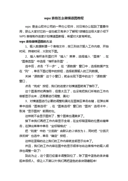
wps表格怎么做横道图教程wps是金山软件公司的一种办公软件，对日常办公起到了重要作用，那么大家对它的一些功能又有多少了解呢?店铺在这给大家介绍下WPS表格制作进度计划横道图教程，希望对大家有帮助。

wps表格做横道图的方法1、输入数据新建一个表格文件，按三列依次输入工作内容、开始时间、持续时间，大致如下图。

2、插入堆积条形图打开“插入”菜单，选择插入“图表”，在“图表类型”中选择“堆积条形图”，选中后，点击“下一步”。

在“源数据”窗口中，选择数据产生在“列”，单击下图红框中的按钮，选择前面输入的三列数据。

关掉“源数据”这个小窗口，就会出现下图中的这个“源数据”窗口，点击“完成”按钮，我们的进度计划横道图就有了雏形了。

这个图虽然初具雏形，但是太丑了，也没有把我们所有的工作内容都显示出来，还需要进行调整、美化!3、对横道图进行必要的调整和美化在图表区单击右键，在弹出菜单中选择“图表选项”，在“图表选项”窗口的“图例”选项卡中，取消“显示图例”前面的勾。

这样就不会显示图例了，整个图表也清爽多了。

接下来我们再把工作内容显示全喽，在坐标轴竖轴的位置右键单击，在弹出菜单中单击“坐标轴格式”，把“刻度”中的“分类数”由默认的2修改为1，同时把“分类次序反转”也选中，单击“确定”按钮，这样在竖轴的边上我们的工作内容就全部显示出来了。

并且，我们的工作内容在图中的显示顺序与右边表格中的输入顺序也调整一致了!到此为止，这个图已经基本调整到位了，除了图中蓝色的条块看起来很烦人、很让人不爽以外!我们再把蓝色的条块隐藏起来!在蓝色条上右键单击，在弹出菜单中点击“数据系列格式”，在下面的窗口中把“边框”和“内部”的图案都设置为“无”，单击“确定”按钮。

这样就很清爽了哈!我们再来把每项工作内容的持续时间显示出来，在红色条块上右键单击，在弹出菜单中点击“数据系列格式”，在弹出窗口“数据标志”选项卡中的“值”前面打勾。

单击“确定”按钮。

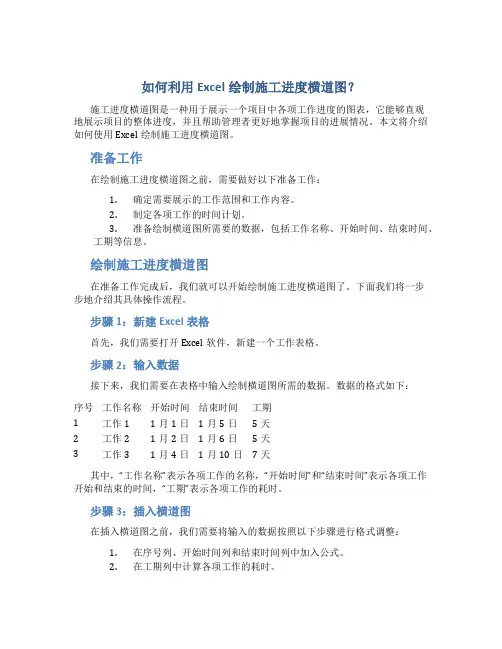
如何利用Excel绘制施工进度横道图？施工进度横道图是一种用于展示一个项目中各项工作进度的图表，它能够直观地展示项目的整体进度，并且帮助管理者更好地掌握项目的进展情况。

本文将介绍如何使用Excel绘制施工进度横道图。

准备工作在绘制施工进度横道图之前，需要做好以下准备工作：1.确定需要展示的工作范围和工作内容。

2.制定各项工作的时间计划。

3.准备绘制横道图所需要的数据，包括工作名称、开始时间、结束时间、工期等信息。

绘制施工进度横道图在准备工作完成后，我们就可以开始绘制施工进度横道图了。

下面我们将一步步地介绍其具体操作流程。

步骤1：新建Excel表格首先，我们需要打开Excel软件，新建一个工作表格。

步骤2：输入数据接下来，我们需要在表格中输入绘制横道图所需的数据。

数据的格式如下：序号工作名称开始时间结束时间工期1 工作1 1月1日1月5日5天2 工作2 1月2日1月6日5天3 工作3 1月4日1月10日7天其中，“工作名称”表示各项工作的名称，“开始时间”和“结束时间”表示各项工作开始和结束的时间，“工期”表示各项工作的耗时。

步骤3：插入横道图在插入横道图之前，我们需要将输入的数据按照以下步骤进行格式调整：1.在序号列、开始时间列和结束时间列中加入公式。

2.在工期列中计算各项工作的耗时。

3.将数据表格中的序号、开始时间、结束时间和工期分别复制到另一个表格中，用于后续绘制横道图所需的数据。

调整完数据格式后，我们就可以开始插入横道图了：1.选中数据表格中的所有数据，包括序号、工作名称、开始时间、结束时间和工期。

2.依次点击“插入”->“条形图”->“横向堆积条形图”。

3.在弹出的“图表工具”中，通过调整图表的样式、颜色和字体等属性，使其更加美观。

绘制完毕后，我们就成功地绘制了施工进度横道图。

施工进度横道图是一种重要的项目管理工具，在项目管理过程中起到了至关重要的作用。

在本文中，我们介绍了如何使用Excel绘制施工进度横道图，并附加了具体的操作步骤。

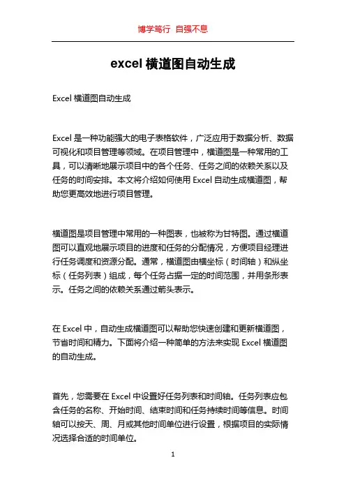
excel横道图自动生成Excel横道图自动生成Excel是一种功能强大的电子表格软件，广泛应用于数据分析、数据可视化和项目管理等领域。

在项目管理中，横道图是一种常用的工具，可以清晰地展示项目中的各个任务、任务之间的依赖关系以及任务的时间安排。

本文将介绍如何使用Excel自动生成横道图，帮助您更高效地进行项目管理。

横道图是项目管理中常用的一种图表，也被称为甘特图。

通过横道图可以直观地展示项目的进度和任务的分配情况，方便项目经理进行任务调度和资源分配。

通常，横道图由横坐标（时间轴）和纵坐标（任务列表）组成，每个任务占据一定的时间范围，并用条形表示。

任务之间的依赖关系通过箭头表示。

在Excel中，自动生成横道图可以帮助您快速创建和更新横道图，节省时间和精力。

下面将介绍一种简单的方法来实现Excel横道图的自动生成。

首先，您需要在Excel中设置好任务列表和时间轴。

任务列表应包含任务的名称、开始时间、结束时间和任务持续时间等信息。

时间轴可以按天、周、月或其他时间单位进行设置，根据项目的实际情况选择合适的时间单位。

接下来，您可以利用Excel中的“条件格式”功能来设置任务的条形表示。

选择任务的起始列和结束列，然后在条件格式中选择“数据条”格式，并调整颜色和样式等参数，使任务的条形图更加美观和易于区分。

然后，您可以使用Excel中的“画图工具”来添加箭头表示任务之间的依赖关系。

在任务列表中选择起始任务和结束任务的单元格，然后在画图工具中选择“箭头”图形，并将箭头指向结束任务的单元格，以表示任务之间的依赖关系。

最后，您可以将任务列表和时间轴的数据导入到Excel中的“数据透视表”中，然后通过数据透视表来生成横道图。

在数据透视表中，将任务列表放置在行区域，时间轴放置在列区域，并将任务持续时间作为数据区域的值。

然后，在数据透视表中选择合适的图表类型（例如簇状条形图），即可自动生成横道图。

通过以上步骤，您就可以在Excel中自动生成横道图了。

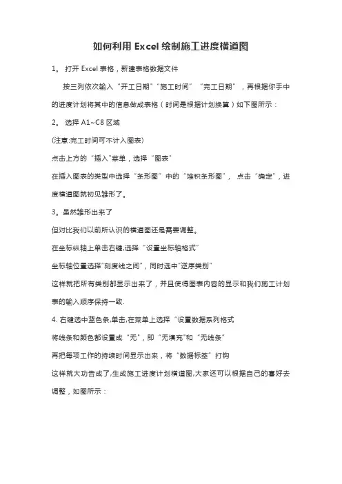
如何利用Excel绘制施工进度横道图
1。

打开Excel表格，新建表格数据文件
按三列依次输入“开工日期"“施工时间”“完工日期”，再根据你手中的进度计划将其中的信息做成表格（时间是根据计划换算）如下图所示：2。

选择A1~C8区域
(注意:完工时间可不计入图表)
点击上方的“插入"菜单，选择“图表"
在插入图表的类型中选择“条形图”中的“堆积条形图”，点击“确定”，进度横道图就初见雏形了。

3。

虽然雏形出来了
但对比我们以前所认识的横道图还是需要调整。

在坐标纵轴上单击右键,选择“设置坐标轴格式”
坐标轴位置选择“刻度线之间”，同时选中“逆序类别”
这样就把所有类别都显示出来了，并且使得图表内容的显示和我们施工计划表的输入顺序保持一致.
4. 右键选中蓝色条,单击,在菜单上选择“设置数据系列格式
将线条和颜色都设置成“无"，即“无填充"和“无线条”
再把每项工作的持续时间显示出来，将“数据标签”打钩
这样就大功告成了,生成施工进度计划横道图,大家还可以根据自己的喜好去调整，如图所示：。

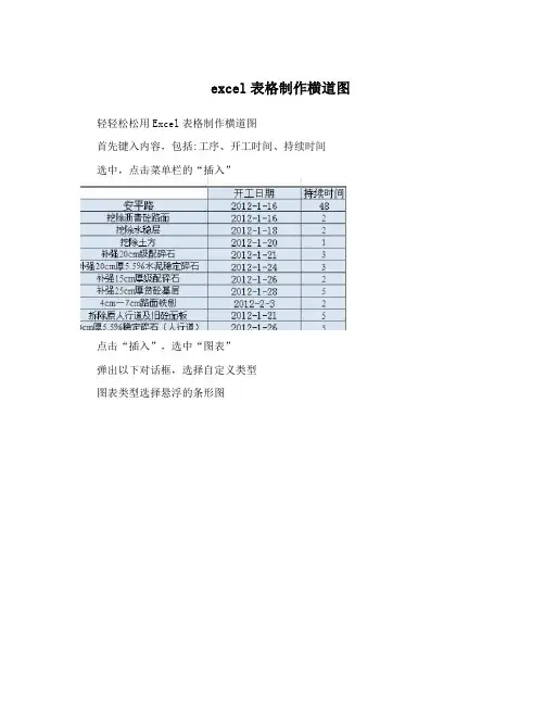
excel表格制作横道图轻轻松松用Excel表格制作横道图首先键入内容，包括:工序、开工时间、持续时间选中，点击菜单栏的“插入”点击“插入”，选中“图表”弹出以下对话框，选择自定义类型图表类型选择悬浮的条形图specifies a method of screening method for the determination of fineness of starch this standard applies to dried into a powder of refined starch. 1, definitions and principles of fineness of starch: starch samples sample screening samples obtained by dividing the weight of the sieve. To sample by dividing the weight of the sieve the sample weight expressed as a percentage of the original weight. Principle: the samples with a sample screen screening, get the sample by dividing the weight of the sieve. 2, instruments and scales: the precision of 0.1g. Sample screen: screen number 100. Step 3, analysis sample preparation: samples should be fully mixed. Sample volume: mix weighing the sample 50g, accurate to 0.1g, evenly pour the sample sieve. Screening: shake the sample sieve evenly, until the screen down so far. Carefully pour out the sample sieve residue on weighing, accurate to 0.1g. Determination of the number: measured on the same sample twice. 4, theresults of the calculation method applied to sample by sample sieve weight expressed as a percentage of the original weight of the sample, as in the formula: x--sample size,%; MO--the original weight of the sample, g; Sift the ML--sample weight of residue on the sieve, g. Such as poor meets the requirements, take the arithmetic mean of the second determination as a result. Results one decimal. 6.2 allowing differential analyst simultaneously or in quick succession for the second determination, the absolute value在这里可以打入标题、选择是否要网格线完成后，得到下图点击Y轴，弹出对话框specifies a method of screening method for the determination of fineness of starch this standard applies to dried into a powder of refined starch. 1, definitions and principles of fineness of starch: starch samples sample screening samples obtained by dividing the weight of the sieve. To sample by dividing the weight of the sieve the sample weight expressed as a percentage of the original weight. Principle: the samples with a sample screen screening, get the sample by dividing the weight of the sieve. 2, instruments and scales: the precision of 0.1g. Sample screen: screen number 100. Step 3, analysis sample preparation: samples should be fully mixed. Sample volume: mix weighing the sample 50g, accurate to 0.1g, evenly pour the sample sieve. Screening: shake the sample sieve evenly, until the screen down so far. Carefully pour out the sample sieve residue on weighing, accurate to 0.1g. Determination of the number: measured on the same sample twice. 4, the results of the calculation method applied to sample by sample sieve weight expressed as a percentage of the original weight of the sample, as in the formula: x--sample size,%; MO--the original weight of the sample, g; Sift the ML--sample weight of residue on the sieve, g. Such as poor meets the requirements, take the arithmetic mean of the seconddetermination as a result. Results one decimal. 6.2 allowing differential analyst simultaneously or in quick succession for the second determination, the absolute value选中“分类次序反转”修改一下字体specifies a method of screening method for the determination of fineness of starch this standard applies to dried into a powder of refined starch. 1, definitions and principles of fineness of starch: starch samples sample screening samples obtained by dividing the weight of the sieve. To sample by dividing the weight of the sieve the sample weight expressed as a percentage of the original weight. Principle: the samples with a sample screen screening, get the sample by dividing the weight of the sieve. 2, instruments and scales: the precision of 0.1g. Sample screen: screen number 100. Step 3, analysis sample preparation: samples should be fully mixed. Sample volume: mix weighing the sample 50g, accurate to 0.1g, evenly pour the sample sieve. Screening: shake the sample sieve evenly, until the screen down so far. Carefully pour out the sample sieve residue on weighing, accurate to 0.1g. Determination of the number: measured on the same sample twice. 4, the results of the calculation method applied to sample by sample sieve weight expressed as a percentage of the original weight of the sample, as in the formula: x--sample size,%; MO--the original weight of the sample, g; Sift the ML--sample weight of residue on the sieve, g. Such as poor meets the requirements, take the arithmetic mean of the second determination as a result. Results one decimal. 6.2 allowingdifferential analyst simultaneously or in quick succession for the second determination, the absolute value点击X轴，弹出对话框修改字体大小修改刻度的最小值，注意“最小值”必须跟“基底(X平面)交叉于(C)”数值保持一致specifies a method of screening method for the determination of fineness of starch this standard applies to dried into a powder of refined starch. 1, definitions and principles of fineness of starch:starch samples sample screening samples obtained by dividing the weight of the sieve. To sample by dividing the weight of the sieve the sample weight expressed as a percentage of the original weight. Principle: the samples with a sample screen screening, get the sample by dividing the weight of the sieve. 2, instruments and scales: the precision of 0.1g. Sample screen: screen number 100. Step 3, analysis sample preparation: samples should be fully mixed. Sample volume: mix weighing the sample 50g, accurate to 0.1g, evenly pour the sample sieve. Screening: shake the sample sieve evenly, until the screen down so far. Carefully pour out the sample sieve residue on weighing, accurate to 0.1g. Determination of the number: measured on the same sample twice. 4, the results of the calculation method applied to sample by sample sieve weight expressed as a percentage of the original weight of the sample, as in the formula: x--sample size,%; MO--the original weight of the sample, g; Sift the ML--sample weight of residue on the sieve, g. Such as poor meets the requirements, take the arithmetic mean of the second determination as a result. Results one decimal. 6.2 allowingdifferential analyst simultaneously or in quick succession for the second determination, the absolute value确定后得到下图，调整一下大小，就OK啦用excel制作横道图就是这么简单，你也可以试试～specifies a method of screening method for the determination of fineness of starch this standard applies to dried into a powder of refined starch. 1, definitions and principles of fineness of starch: starch samples sample screening samples obtained by dividing the weight of the sieve. To sample by dividing the weight of the sieve the sample weight expressed as a percentage of the original weight. Principle: the samples with a sample screen screening, get the sample by dividing the weight of the sieve. 2, instruments and scales: the precision of 0.1g. Sample screen: screen number 100. Step 3, analysis sample preparation: samples should be fully mixed. Sample volume: mix weighing the sample 50g, accurate to 0.1g, evenly pour the sample sieve. Screening: shake the sample sieve evenly, until the screen down so far. Carefully pour out the sample sieve residue on weighing, accurate to 0.1g. Determination of the number: measured on the same sample twice. 4, the results of the calculation method applied to sample by sample sieve weight expressed as a percentage of the original weight of the sample,as in the formula: x--sample size,%; MO--the original weight of the sample, g; Sift the ML--sample weight of residue on the sieve, g. Such as poor meets the requirements, take the arithmetic mean of the second determination as a result. Results one decimal. 6.2 allowing differential analyst simultaneously or in quick succession for the second determination, the absolute value。

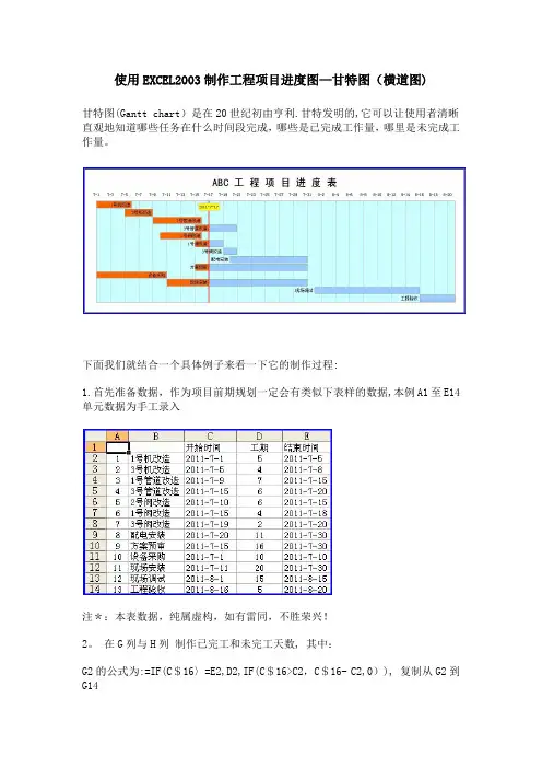
使用EXCEL2003制作工程项目进度图—甘特图（横道图)甘特图(Gantt chart）是在20世纪初由亨利.甘特发明的,它可以让使用者清晰直观地知道哪些任务在什么时间段完成，哪些是已完成工作量，哪里是未完成工作量。

下面我们就结合一个具体例子来看一下它的制作过程:1.首先准备数据，作为项目前期规划一定会有类似下表样的数据,本例A1至E14单元数据为手工录入注＊：本表数据，纯属虚构，如有雷同，不胜荣兴！2。

在G列与H列制作已完工和未完工天数, 其中：G2的公式为:=IF(C＄16〉=E2,D2,IF(C＄16>C2，C＄16- C2,0）), 复制从G2到G14H2的公式为:=IF（C$16〈=C2,D2，IF（C＄16<E2,E2—C＄16+1，0）), 复制从H2到H143. 继续加数据，B16到C18为手工输入。

D16、D17、D18分别等于C16、C17、C18。

然后将D16：D18单元格格式由日期改成数值型。

至于为什么需要做这部分数据，后文有述. 目前只需要知道EXCEL的日期数据,从本质上来讲就是一个整数。

4. 开始作图。

首先同时选择B1到C14 和 G1到H14 两个区域。

注意数据区域的选择是，先选中B1到C14，然后按住Ctrl键不放，再选择G1到H1。

5. 然后，单击工具栏上的图表向导，选择“条形图” 中的“堆积条形图”,然后直接点完成。

6。

如果您操作正确的话，出来的图应该是下面这个样子。

在右侧的“图列”上按鼠标右键，选“清除”,同时将图表区拉长拉宽一些，因为这个图可能会有些大。

7。

拖动图表大小差不多是从19行到42行，从A列到P列（行高和列宽为默认），这里顺便提一下图表上的一些元素名称，下文会经常用到。

8。

在图表区上按鼠标右键-—〉图表区格式 --> 在"字体"页选字号为9—-〉去除自动缩放前的钩选--> 确定9。

绘图区域内，选中蓝色的数据系列 --> 右键——〉数据系列格式10。

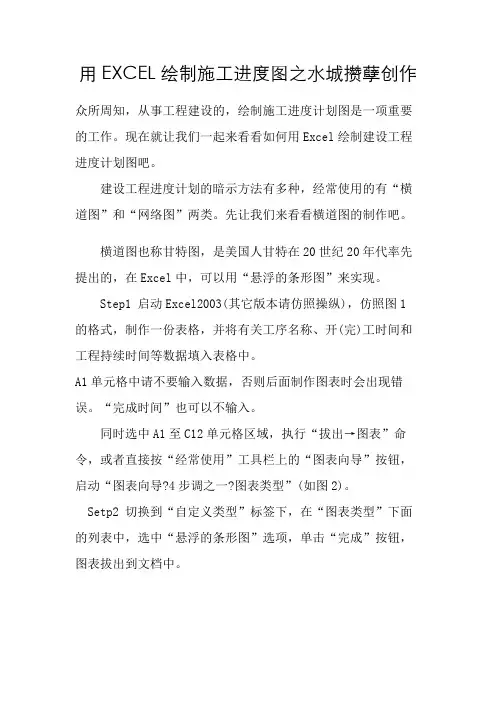
用EXCEL绘制施工进度图之水城攒孽创作众所周知，从事工程建设的，绘制施工进度计划图是一项重要的工作。

现在就让我们一起来看看如何用Excel绘制建设工程进度计划图吧。

建设工程进度计划的暗示方法有多种，经常使用的有“横道图”和“网络图”两类。

先让我们来看看横道图的制作吧。

横道图也称甘特图，是美国人甘特在20世纪20年代率先提出的，在Excel中，可以用“悬浮的条形图”来实现。

Step1 启动Excel2003(其它版本请仿照操纵)，仿照图1的格式，制作一份表格，并将有关工序名称、开(完)工时间和工程持续时间等数据填入表格中。

A1单元格中请不要输入数据，否则后面制作图表时会出现错误。

“完成时间”也可以不输入。

同时选中A1至C12单元格区域，执行“拔出→图表”命令，或者直接按“经常使用”工具栏上的“图表向导”按钮，启动“图表向导?4步调之一?图表类型”(如图2)。

Setp2 切换到“自定义类型”标签下，在“图表类型”下面的列表中，选中“悬浮的条形图”选项，单击“完成”按钮，图表拔出到文档中。

然后用鼠标双击图表的纵坐标轴，打开“坐标轴格式”对话框，切换到“刻度”标签下，选中“分类次序反转”选项；再切换到“字体”标签下，将字号设置小一些，确定返回。

小技巧：经过此步操纵，图表中有关“工序名称”就按开工顺序从上到下排列了，这样更符合我们的实际情况。

Step3 仿照上面的操纵，打开横坐标轴的“坐标轴格式”对话框，在“刻度”标签中，将“最小值”和“交叉于”后面的方框中的数值都设置为“37994”(即日期2004-1-8的序列值，具体应根据实际情况确定)；同时，也在“字体”标签中，将字号设置小一些，确定返回。

调整好图表的大小和长宽比例，一个规范的横道图制作完成(图3)。

你也可以利用相应的设置对话框，修改图表的格式、颜色等设置，感兴趣的读者请自己练习设置。

电子表格制作横道图方法　1.将图表中的部分图形“隐藏”起来 如果为了实现某种特殊的图表效果，需要将图表中的部分图形“隐藏”起来，除了将该系列删除外（有时候这种方法不能达到所需要的效果），还可以通过下面的方法来实现。

步骤1：在图表中选中需要“隐藏”的图表图形。

步骤2：切换到“图表工具／格式”菜单选项卡中。

步骤3：单击“形状样式”组中的“形状填充”下拉按钮，在随后出现的下拉列表中，选择“无填充颜色”选项即可。

2.调整图表图形宽度 对于柱形、条形等图表来说，如果用户觉得图形的宽度不太合适，可以通过下面的操作来进行调整。

步骤1：在图表中选中相应的图表图形。

步骤2：右击鼠标，在随后出现的快捷菜单中，选择“设置数据点格式”选项，打开“设置数据点格式”对话框。

步骤3：在“系列选项”标签中，结合“即看即所得”功能，调整“分类间距”下面的数值至合适值后，单击“关闭”返回即可。

【实战练习】 下面，我们实战演练制作如图1所示的施工进度横道图的具体过程。

图1 1．建立图表 步骤1：启动Excel 2007，在某个工作表中，输入施工进度数据，如图2所示。

图2 步骤2：选中A2：C14单元格区域，用“条形图—堆积条形图”图表类型建立一个图表，如图3所示。

图3 2.格式化图表 步骤1：在图表中，单击“开始日期”系列图形，选中它，右击鼠标，在随后出现的快捷菜单中，选择“设置数据点格式”选项，打开“设置数据点格式”对话框。

步骤2：激昂“填充”和“边框颜色”均设置为“无”，单击“关闭”返回。

步骤3：切换到“图表工具/布局”菜单选项卡中，选中图表中的横轴，然后单击“当前所选内容”组中的“设置所选内容格式”按钮，打开“设置坐标轴格式”对话框。

步骤4：在“坐标轴选项”栏目中，选中“最小值/固定”项目，并在后面的方框中输入“39414”；选中“最大值/固定”项目，并在后面的方框中输入数值“39640”；选中“主要刻度单位/固定”项目，并在后面的方框中输入数值“20”；选中“次要刻度单位/固定”项目，并在后面的方框中输入数值“5”.其他采用默认格式。

Excel与横道图在建筑工程中，横道图是我们一个陌生不过的东西。

其实横道图又称为甘特图。

画横道图的工具或者软件虽然是不少，比如：Microsoft的project、ccproject网络图绘制软件、甚至也可以用Microsoft的Word来作图。

现在介绍下如何用Microsoft的Excel来画横道图是怎样操作的。

（这里我是用Excel 2013来演示操作，如果是比较低版本的Excel来画横道图是有些设置不太相同的，比如Excel 2003以下的版本）接下来，我们一起来学习下怎样在Excel里生成横道图。

首先打开我们需要的软件Excel，把需要的开始日期、结束日期和天数输入单元格里（这里以Excel 2013为例）选择数据区域中的选择任一个单元格，在功能区中选择“插入——更多图形条形图——堆积条形图”选择堆积条形图确认后，接着就自动生成了条形图。

看到的这个条形图还不是我们想要的，别急，我们继续接下去完善。

选择刚刚弹出的条线图——选择图标工具的设计——选择数据——把结束日期删掉——确认。

这时，条形图里结束日期的进度条被我们删掉了。

选择开始日期——右击——选择设置数据系列格式（Excel 2003等一下版本，双击开始日期即可）然后，点击油漆桶——填充——选择无填充，此时我们会看到开始日期的进度条会变成透明的。

到这里，终于达到事半功倍了。

眼看就要大功告成了。

别高兴这么快，我们继续下一步调整。

选择图表选项——垂直（类别）轴选择坐标轴选项——逆序类别前面的方框把勾打上。

这里说明一下，坐标轴选项下的最小值和最大值都是填数值的，实际要填上的是我们工程的最早的开工日期和竣工验收的日期（这个是基于低版本的做法）Excel 2007以上的要填入日期的序列数。

序列数的获取方法有很多，比如我以2014-10-3（最小值）和2015-1-2（最大值）；选择2014-10-3单元格把它的属性”日期“改为”常规“，这样单元格就会变成41915；同理2015-1-2也就变成42008了。