量子力学_陈洪_电子教案第8章一维量子化体系
- 格式:ppt
- 大小:487.50 KB
- 文档页数:30

量子力学简明教程授课教案第一章:量子力学概述1.1 量子力学的发展历程了解量子力学的历史背景,包括普朗克的量子假说、爱因斯坦的光量子理论、波粒二象性等。
学习量子力学的基本原理,如波函数、薛定谔方程、海森堡不确定性原理等。
探索量子力学在原子、分子、固体物理等领域中的应用。
第二章:波函数与薛定谔方程2.1 波函数的概念学习波函数的定义和数学表达,了解波函数的物理意义和作用。
掌握波函数的归一化条件和物理意义。
2.2 薛定谔方程推导薛定谔方程,并了解其在量子力学中的重要性。
学习一维势阱、势垒和量子隧穿等模型。
第三章:量子力学的基本概念3.1 量子态的叠加与测量学习量子态的叠加原理,了解测量对量子态的影响。
探讨量子纠缠和量子超位置等现象。
3.2 量子力学的基本数学工具学习算符的概念和运算规则,了解算符在量子力学中的应用。
掌握态空间、算符表示和测量理论等基本概念。
第四章:原子和分子的量子力学4.1 氢原子的量子力学学习氢原子的薛定谔方程和解空间波函数。
探讨能级、能级跃迁和光谱线等现象。
4.2 多电子原子的量子力学学习多电子原子的薛定谔方程和电子间的相互作用。
探讨原子轨道、电子云和原子性质等概念。
第五章:固体物理中的量子力学5.1 晶体的量子力学学习晶体的周期性边界条件和布拉格子模型。
探讨能带结构、能带间隙和电子在晶体中的行为等概念。
5.2 量子阱和量子线学习量子阱和量子线的结构及其电子性质。
探讨量子阱中的量子态和量子线中的电子传输等现象。
第六章:量子力学与经典力学的比较6.1 经典力学的局限性探讨经典力学在描述微观粒子行为时的不足之处。
学习量子力学与经典力学在概念和方法上的差异。
6.2 量子力学的非经典特性探讨量子力学的非经典特性,如波粒二象性、量子纠缠等。
学习量子力学与经典力学在预测和解释现象上的不同。
第七章:量子力学与相对论的关系7.1 狭义相对论的基本概念复习狭义相对论的基本原理,如时空相对性、质能等价等。

《量子力学简明教程》授课教案一、第1章:量子力学导论1.1 课程简介介绍量子力学的发展历程及其在现代物理学中的重要性。
解释量子力学与经典力学的区别和联系。
1.2 教学目标让学生了解量子力学的历史背景和发展。
让学生理解量子力学的基本概念和原理。
1.3 教学内容量子力学的历史背景和发展。
量子力学的基本概念:波函数、薛定谔方程、测量问题等。
1.4 教学方法采用讲授法,辅以案例分析、讨论等方式,帮助学生理解和掌握基本概念。
二、第2章:一维势阱与量子束缚态2.1 课程简介研究一维势阱中粒子的行为,探讨束缚态和散射态的性质。
2.2 教学目标让学生掌握一维势阱的基本性质和量子束缚态的解法。
让学生了解束缚态和散射态的区别。
2.3 教学内容一维势阱的基本性质:能级、能态、束缚态和散射态。
量子束缚态的解法:数学表达式、图形表示、解的存在性等。
2.4 教学方法采用数值计算、图形演示等方法,帮助学生直观地理解一维势阱的性质。
通过实例分析,让学生掌握量子束缚态的解法。
三、第3章:势垒穿透与量子隧道效应3.1 课程简介研究在势垒作用下,粒子穿过势垒的概率问题,探讨量子隧道效应的性质。
3.2 教学目标让学生了解势垒穿透的条件和量子隧道效应的物理意义。
让学生掌握量子隧道效应的数学表达式和应用。
3.3 教学内容势垒穿透的条件:入射粒子的能量、势垒的宽度、形状等。
量子隧道效应的物理意义和数学表达式。
量子隧道效应的应用:纳米技术、扫描隧道显微镜等。
3.4 教学方法采用数值计算、图形演示等方法,帮助学生直观地理解势垒穿透和量子隧道效应。
通过实例分析,让学生掌握量子隧道效应的数学表达式和应用。
四、第4章:哈密顿算符与量子平均值4.1 课程简介引入哈密顿算符的概念,研究量子系统的能量本征值和本征态。
探讨量子平均值的计算方法及其在实际问题中的应用。
4.2 教学目标让学生理解哈密顿算符的概念及其物理意义。
让学生掌握量子平均值的计算方法及其应用。
量子力学简明教程授课教案第一章:量子力学概述1.1 量子力学的发展历程1.2 量子力学的基本概念1.3 量子力学与经典力学的比较第二章:波函数与薛定谔方程2.1 波函数的概念2.2 薛定谔方程的建立2.3 薛定谔方程的求解方法第三章:量子态的叠加与测量3.1 量子态的叠加原理3.2 量子态的测量3.3 测量结果的概率解释第四章:一维势阱与量子束缚态4.1 一维势阱的经典问题4.2 量子束缚态的能量与波函数4.3 束缚态的跃迁与吸收、发射现象第五章:量子力学在原子物理中的应用5.1 氢原子的能级与光谱5.2 多电子原子的能级结构5.3 激光原理与激光器第六章:量子力学在分子物理中的应用6.1 分子轨道理论的基本概念6.2 分子轨道的能级与形状6.3 分子间相互作用与化学键第七章:量子力学在凝聚态物理中的应用7.1 晶体结构的基本概念7.2 电子在晶体中的能带结构7.3 半导体与超导体的量子性质第八章:量子力学在量子计算中的应用8.1 量子比特与量子电路8.2 量子门的操作与量子计算的基本原理8.3 量子算法与量子计算机的优势第九章:量子力学在量子通信中的应用9.1 量子态的传输与量子纠缠9.2 量子密钥分发与量子通信的安全性9.3 量子通信的未来发展与应用第十章:量子力学在粒子物理中的应用10.1 粒子物理的基本概念10.2 量子场论的基本原理10.3 粒子的产生与衰变过程重点和难点解析一、量子力学的发展历程难点解析:理解量子力学与经典力学的本质区别,以及量子概念的引入对物理学带来的革命性变革。
二、波函数与薛定谔方程难点解析:解薛定谔方程的技巧,特别是束缚态和散射态的求解,以及如何从解中提取物理信息。
三、量子态的叠加与测量难点解析:量子测量理论,包括测量结果的概率解释和量子纠缠现象。
四、一维势阱与量子束缚态难点解析:理解量子束缚态的概念,以及如何计算束缚态的能量和波函数。
五、量子力学在原子物理中的应用难点解析:如何用量子力学解释氢原子的光谱线系列,以及激光产生的物理过程。
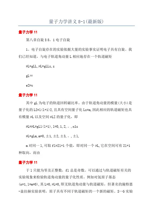
量子力学讲义8-1(最新版)量子力学11第八章自旋§8。
1电子自旋1、电子自旋存在的实验依据大量的实验事实证明电子具有自旋。
我们已经知道,与电子轨道角动量L相应地存在一个轨道磁矩µL=gLL,µL=gLLz,zgL≡e2µc量子力学11其中gL为电子的轨道回转磁比率。
由于轨道角动量的模量(大小)是量子化的L2=l(l+1)2,且具有空间量子化Lz=m,因此相应的轨道磁矩也具有模量µL以及空间µLZ的量子化,即µL=µL=gLl(l+1),l=0,1,2,。
,n1zµL=gLm,m=0,±1,±2,±3,。
,±l,m对同一l,可取fl=2l+1个值,即对同一个µL,它在空间可有2l+1种取向,而由量子力学11于l只能为零及正整数,fl总是奇数。
可以通过与轨道磁矩有关的实验现象来检验轨道角动量的量子化性质。
例如对氢原子基态(n=1,l=m=0),其L=0,µL=0,即无轨道角动量与轨道磁矩,但著名的施特恩-盖拉赫实验表明,原子具有不同于轨道磁矩的一个新的磁矩。
S—G实验如下图所示,由K源射出的处于S态(基态)的氢原子束经过狭缝和不均匀磁场照射到底片上,结果发现射线束方向发生偏转,分裂成两条分立的线,这说明氢原子有磁矩,在非均匀磁场的作用下受到力的作用而发生偏转。
量子力学11zNBBS(8。
1)SternGerlach实量子力学11由于这是处于基态的氢原子,轨道角动量为零,基态氢原子的磁矩不可能由轨道角动量产生,故是一种新的磁矩。
此外,由于实验上发现只有两条谱线,因而这种磁矩在磁场中只有两种取向,是空间量子化的,而且只取两个值。
若原子具有磁矩µ,它在z方向上的外磁场B中的势能为θ(3)为外磁场B与原子磁矩µ之间的夹角。
U=µB=µBzcoθ量子力学11而原子因磁矩µ的存在,在Z方向上受到的力为BzU=µcoθFz=(4)zz实验表明,这时分裂出来的两条谱线分别对应于coθ=+1和coθ=1两个值。
Lecture2Quantum mechanics in one dimensionQuantum mechanics in1d:Outline1Unbound statesFree particlePotential stepPotential barrierRectangular potential well2Bound statesRectangular potential well(continued)δ-function potential3Beyond local potentialsKronig-Penney model of a crystalAnderson localizationi ∂tΨ(x,t)=− 2∂2x2mΨ(x,t)For V=0Schr¨o dinger equation describes travelling waves.Ψ(x,t)=A e i(kx−ωt),E(k)= ω(k)= 2k2 2mwhere k=2πλwithλthe wavelength;momentum p= k=hλ.Spectrum is continuous,semi-infinite and,apart from k=0,has two-fold degeneracy(right and left moving particles).i ∂tΨ(x,t)=− 2∂2x2mΨ(x,t)Ψ(x,t)=A e i(kx−ωt)For infinite system,it makes no sense tofix wave function amplitude,A,by normalization of total probability.Instead,fix particleflux:j=−2m(iΨ∗∂xΨ+c.c.)j=|A|2 km=|A|2pmNote that definition of j follows from continuity relation,∂t|Ψ|2=−∇·jThe Fourier transform of a normalized Gaussian wave packet,ψ(x)= 12πα 1/4e ik0x e−x24α.(moving at velocity v= k0/m)is also a Gaussian,ψ(k)= 2απ 1/4e−α(k−k0)2,Although we can localize a wave packet to a region of space,this has been at the expense of having some width in k.For the Gaussian wave packet,∆x = [x − x ]2 1/2≡ x 2 − x 2 1/2=√α,∆k =1√4αi.e.∆x ∆k =12,constant.In fact,as we will see in the next lecture,the Gaussian wavepacket has minimum uncertainty ,∆p ∆x = 2Stationary form of Schr¨o dinger equation,Ψ(x,t)=e−iEt/ ψ(x):− 2∂2x2m+V(x) ψ(x)=Eψ(x)As a linear second order differential equation,we must specify boundary conditions on bothψand its derivative,∂xψ. As|ψ(x)|2represents a probablility density,it must be everywherefinite⇒ψ(x)is alsofinite. Sinceψ(x)isfinite,and E and V(x)are presumedfinite,so∂2xψ(x)must befinite.⇒bothψ(x)and∂xψ(x)are continuous functions of xFor E >V 0,both k <and k >=2m (E −V 0)are real,and j i = k <m,j r =|r |2 k <m,j t =|t |2 k >mDefining reflectivity,R ,and transmittivity,T ,R =reflected flux incident flux,T =transmitted flux incident flux R =|r |2=k <−k >k <+k >2,T =|t |2k >k <=4k <k >(k <+k >)2,R +T =1For E <V 0, k >=2m (E −V 0)becomes pure imaginary,wavefunction,ψ>(x ) te −|k >|x ,decays evanescently,andj i = k <m,j r =|r |2 k <m,j t =0Beam is completely reflected from barrier,R =|r |2= k <−k >k <+k >2=1,T =0,R +T =1Transmission across a potential barrier–prototype for generic quantum scattering problem dealt with later in the course. Problem provides platform to explore a phenomenon peculiar to quantum mechanics–quantum tunneling.Wavefunction parameterization:ψ1(x)=e ik1x+r e−ik1x x≤0ψ2(x)=A e ik2x+B e−ik2x0≤x≤aψ3(x)=t e ik1x a≤xwhere k1=√2mE and k2= 2m(E−V0).Continuity conditions onψand∂xψat x=0and x=a,1+r=A+BAe ik2a+Be−ik2a=te ik1a, k1(1−r)=k2(A−B)k2(Ae ik2a−Be−ik2a)=k1te ik1aSolving for transmission amplitude,t=2k1k2e−ik1a2k1k2cos(k2a)−i(k21+k22)sin(k2a)which translates to a transmissivity ofT=|t|2=11+14 k1k2−k2k1 2sin2(k2a) and reflectivity,R=1−T(particle conservation).but penetrates,barrier region–quantumUnbound particles:tunnelingAlthough tunneling is a robust,if uniquely quantum,phenomenon,it is often difficult to discriminate from thermal activation.Experimental realization provided by Scanning TunnelingMicroscope(STM)Quantum mechanical scattering in three-dimensions In three dimensions,plane wave can be decomposed intosuperposition of incoming and outgoing spherical waves: If V(r)short-ranged,scattering wavefunction takes asymptotic form,e i k·r=i2k∞ =0i (2 +1) e−i(kr− π/2)r−S (k)e i(kr− π/2)r P (cosθ)Quantum mechanics in1d:bound states1Rectangular potential well(continued)2δ-function potentialFor a potential well,we seek bound state solutions with energies lying in the range−V0<E<0.Symmetry of potential⇒states separate into those symmetric and those antisymmetric under parity transformation,x→−x. Outside well,(bound state)solutions have form√−2mE>0ψ1(x)=Ceκx for x>a, κ=In central well region,general solution of the formψ2(x)=A cos(kx)or B sin(kx), k= 2m(E+V0)>0Uncertainty relation,∆p∆x>h,shows that confinement by potential well is balance between narrowing spatial extent ofψwhile keeping momenta low enough not to allow escape.In fact,one may show(exercise!)that,in one dimension,arbitrarily weak binding always leads to development of at least one bound state.In higher dimension,potential has to reach critical strength to bind a particle.Forδ-function potential V(x)=−aV0δ(x),− 2∂2x2m−aV0δ(x) ψ(x)=Eψ(x)(Once again)symmetry of potential shows that stationary solutions of Schr¨o dinger equation are eigenstates of parity,x→−x.States with odd parity haveψ(0)=0,i.e.insensitive to potential.Quantum mechanics in1d:beyond local potentials1Kronig-Penney model of a crystal2Anderson localizationKronig-Penney model provides caricature of(one-dimensional) crystal lattice potential,∞ n=−∞δ(x−na)V(x)=aV0Since potential is repulsive,all states have energy E>0. Symmetry:translation by lattice spacing a,V(x+a)=V(x). Probability density must exhibit same translational symmetry, |ψ(x+a)|2=|ψ(x)|2,i.e.ψ(x+a)=e iφψ(x).In region(n−1)a<x<na,general solution of Schr¨o dinger equation is plane wave like,ψn(x)=A n sin[k(x−na)]+B n cos[k(x−na)]√2mEwith k=Imposing boundary conditions onψn(x)and∂xψn(x)and requiring ψ(x+a)=e iφψ(x),we can derive a constraint on allowed k values (and therefore E)similar to quantized energies for bound states.Rearranging equations(1)and(2),and using the relations A n+1=e iφA n and B n+1=e iφB n,we obtaincosφ=cos(ka)+maV02k sin(ka)Since cosφcan only take on values between−1and1,there are2k2Example:Naturally occuring photonic crystals “Band gap”phenomena apply to any wave-like motion in a periodicsystem including light traversing dielectric media,e.g.photonic crystal structures in beetles and butterflies!Band-gaps lead to perfect reflection of certain frequencies.Anderson localizationWe have seen that even a weak potential can lead to the formationof a bound state.However,for such a confining potential,we expect high energystates to remain unbound.Curiously,and counter-intuitively,in1d a weak extended disorderpotential always leads to the exponential localization of allquantum states,no matter how high the energy!First theoretical insight into the mechanism of localization wasachieved by Neville Mott!。
西南大学物理专业《量子力学》教学大纲(2006年6月)一、课程说明1.课程类型量子力学基础是重庆市高等教育物理教育专业的一门专业必修课。
2.课程特点量子力学是研究微观体系,探讨微观粒子(分子、原子、原子核)的结构及运动规律的科学。
它不仅是物理学的基础理论,在物理学科中有广泛的应用,而且在化学、生物学、医学等相关学科和现代技术重视得到广泛的应用。
大量事实证明,离开量子理论,任何一门近代物理学科及相关边缘学科的发展都是不可思议的。
可以毫不夸张地说,没有量子理论的建立,就没有人类的现代物质文明。
正由于量子力学这门课程的重要性,它一直作为物理教育专业的主干基础课之一。
该课程有以下几个特点:(1)注重基础理论与实验事实之间的统一,并用严格的量子力学理论对实验事实给予正确的解释。
(2)强调微观的物质性和行为统计规律性,注意阐明量子力学与经典理论之间的差别和相互关系。
(3)强调理论的系统性、逻辑性,并用比较严密的教学论证来加深对物理规律和物理现象的理解,但不纯粹数学化。
(4)注重基础理论与现代物理科学发展前沿、最新科技成果的联系,也注意与相关学科联系。
3、教学目的通过量子力学基础课程的学习,应试学生掌握基本概念、基本理论、处理具体问题的基本方法,并能用所学的理论、方法对物理现象,特别是科学最新发现的新现象给予正确理解,培养学生形象思维能力和逻辑思维能力及创新意识。
4、课程安排我们将量子力学课程分为两个部分。
第一部分(1-8章)为必修内容,共计72学时,主要讲授量子力学的基本原理和方法,包括量子力学的实验基础、基本原理、方法以及一些基本的量子力学例子;第二部分(9-11章)为选修内容,共计24学时,主要使学生了解量子力学的进展。
二、教学内容和要求第一章量子论基础(4学时)1、教学内容§1.1 黑体辐射与普朗克的能量子;§1.2 光电效应与爱因斯坦的光量子;§1.3 康普顿效应;§1.4 原子结构与玻尔的量子论;§1.5 德布罗意的物质波.2、教学要求掌握量子力学建立的关键实验基础和物质波假说;掌握原子结构玻尔量子论的成就和缺陷。
量子力学简明教程授课教案一、引言1. 课程背景和目的2. 量子力学的重要性3. 课程结构和安排二、量子概念的诞生1. 经典物理学的局限性2. 黑体辐射和普朗克的量子假设3. 玻尔的原子模型4. 量子观念的逐步确立三、波函数和薛定谔方程1. 波函数的引入2. 薛定谔方程的建立3. 量子态的叠加和测量4. 实例分析:氢原子的能级和光谱四、量子力学的基本概念1. 算符和测量2. 量子数的意义3. 泡利不相容原理4. 洪特规则5. 实例分析:电子的轨道和自旋五、原子和分子的量子力学1. 电子云和概率密度2. 势能曲线和能级图3. 原子和分子的光谱4. 实例分析:激光和光谱仪的应用5. 量子力学在化学键理论中的应用六、量子力学与固体物理1. 晶体的量子力学描述2. 能带理论和半导体物理3. 超导性和量子遂穿现象4. 实例分析:量子点和水分子在固体中的行为七、粒子物理学与量子场论1. 基本粒子和量子场论2. 标准模型的构建3. 量子色动力学和电弱相互作用4. 实例分析:粒子加速器和LHC实验八、量子信息和量子计算1. 量子比特和量子纠缠2. 量子门和量子操作3. 量子算法和量子优势4. 实例分析:量子加密和量子通信九、量子力学在生物学中的应用1. 量子生物学概述2. 光合作用和量子效率3. 生物分子和量子干涉4. 实例分析:量子态在酶催化和DNA测序中的应用十、量子力学在未来科技的发展趋势1. 量子模拟和量子计算机的发展2. 量子通信和量子网络的构建3. 量子传感器的应用前景4. 实例分析:量子科技在医疗、能源和交通领域的潜在影响十一、量子力学在量子模拟中的应用1. 量子模拟器的原理与构造2. 模拟复杂量子系统的方法3. 量子模拟在材料科学中的应用4. 实例分析:量子模拟在高温超导体研究中的应用十二、量子力学与量子光学1. 量子光学的基本原理2. 光的量子化与量子态的操控3. 量子干涉与量子纠缠4. 实例分析:量子隐形传态与量子密钥分发十三、量子力学与量子化学1. 量子化学的基本方法2. 分子轨道理论与量子化学计算3. 量子力学在化学反应动力学中的应用4. 实例分析:量子化学软件与实验结果的对比分析十四、量子力学在核物理中的应用1. 量子力学的核物理背景2. 量子态在核反应中的演化3. 量子力学在核磁共振成像中的应用4. 实例分析:核物理实验中的量子力学解释十五、总结与展望1. 量子力学的重要性和普适性2. 量子力学在现代科技中的关键作用3. 量子力学未来的挑战与发展方向4. 实例分析:结合最新科研成果,展望量子力学的未来发展趋势重点和难点解析1. 量子概念的诞生:理解经典物理学的局限性和量子观念的逐步确立是学习量子力学的基础。