Sociophysics Simulations II Opinion Dynamics

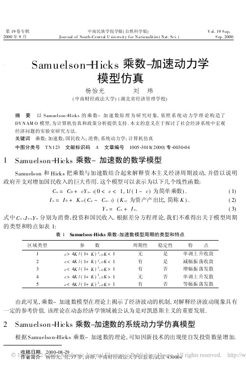
第19卷专辑 中南民族学院学报(自然科学版) Vol.19S up. 2000年9月 Jour nal of South-Central U nivers ity for Nationalities(Nat.Sci.) S ep.2000Samuelson-Hicks乘数-加速动力学模型仿真杨怡光(中南财经政法大学)刘　玮(湖北省经济管理学校)摘　要　以Samuelson-Hicks的乘数-加速数原理为研究对象,依照系统动力学理论构造了DY N AM O模型,为计算机仿真和政策分析提供支持.本文的意义在于探讨了社会经济系统中宏观经济问题的实验室研究方法.关键词　乘数;加速数;国民收入;消费;系统动力学;计算机仿真中图分类号　T N123　文献标识码　A　文章编号　1005-3018(2000)专-0030-041　Samuelson-Hicks乘数-加速数的数学模型Samuelson和Hicks把乘数与加速数结合起来解释资本主义经济周期波动,并借以说明政府开支对增加国民收入的巨大作用.这个模型可以表示为以下几个线性函数:C n=C0+cY n-1(0<c<1,1/(1-c)为简单乘数).(1)I n=I0+K or(C n-C n-1)(K or为资产产出比,简称K).(2)Y n=C n+I n.(3)式中C n、I n、Y n分别为消费、投资和国民收入.根据差分方程理论,我们不难得出关于模型周期的类型和特点如表1:表1　Samuelson-Hicks乘数-加速数模型周期的类型和特点区域类型参 数周期性稳定性特 点1c>4K/(1+K)2,cK<1无是单调上升收敛2c<4K/(1+K)2,cK<1有是减幅振荡收敛3c<4K/(1+K)2,cK>1有否增幅振荡发散4c>4K/(1+K)2,cK>1无否单调上升发散5c<4K/(1+K)2,cK=1有否等幅振荡发散由此可见,乘数-加速数模型在理论上揭示了经济波动的机制,对解释经济波动现象具有一定的参考价值.该理论在动态经济学领域被公认为是对凯恩斯主义的重要发展.2　Samuelson-Hicks乘数-加速数的系统动力学仿真模型根据Samuelso n-Hicks乘数-加速数的理论,可知因新技术的出现使自发投资数量增加.收稿日期　2000-08-29作者简介　杨怡光,男,37岁,讲师,中南财经政法大学信息系,武汉430064这一冲击在经济体系内部通过乘数作用导致国民收入的增加,而国民收入的增长会使人们相应增加消费需求,引致投资便由此而生,并且它对消费需求增加的反应是加速的.加速增加的引致投资又通过乘数关系推动国民收入的更快增长.这又反过来促使引致投资更大的增加.如此循环往复,产量和收入不断增加,表明经济体系处于经济周期的扩张阶段.但由于社会资源有限,当经济扩张达到资源与技术水平所能允许的最大产量极限时,经济体系处于经济周期的峰顶,国民收入已无法增加,消费需求也不再增加,导致投资降至为零.从动态过程看,国民收入在接近顶峰阶段时增长率的逐步下降,消费需求增长率就相应下降,由此而造成投资增长率的更大下降.投资增长率下降最终会使国民收入下降.由此又使消费需求下降,从而导致投资加速减少.反过来通过乘数作用导致国民收入的更快的减少.如此循环往复,国民收入不断下降,经济体系便处于经济周期的收缩或衰退阶段.当经济收缩到由总需求所决定的最低国民收入水平时,经济体系处于经济周期的谷底.由于在收缩阶段长期进行的负投资使闲置资本物品被抵消.为此重置投资成为必要.一旦重置投资出现,乘数作用将使产量和收入上升,加速原理相应发生作用.乘数与加速数的相互作用,会推动经济体系再次处于经济周期的扩张阶段.这意味着新一轮的经济周期重新开始.根据系统动力学原理,我们得出Samuelson-Hicks 乘数-加速动力学模型的流图如图1.图1　乘数-加速数模型系统流图根据Sam uelso n -Hicks 乘数-加速模型的流图,我们利用DYNAM O 语言写出相应的DYNAM O 方程如下:L Y.K=Y.J+DT *(I.JK-C.JK)+G.KA G .K =G .J +RAND ()N Y=589(亿元)R I.KL =C.JK*Kic+Y.K*CLIP(Kiy ,1-C 0,1-C 0,Kiy )+(DK .K -K .K)/T31专辑 杨怡光等:Samuelson -Hicks 乘数-加速动力学模型仿真 R C .KL =AY .K *C 0N Kic =0.4N C0=0.35N Kiy =0.18N T =5L K .K =K .J +DT *I .JK /T A DK .K =DK .J *t +AY .K *Kor N Kor =0.45A AY.K =AY.J+DT *(Y.K-AY.J)/T s N T s =3图2　仿真结果3　实例分析本文以C 语言为工具对该模型进行仿真分析,主要考虑平均消费比例,投资与消费比,投资与收入比,资产调节时间,资产与产出比,收入平滑时间6个因素的变动对整个模型的影响.原始数据为我国1952年以来宏观经济方面的实际指标.如图3,各指标的曲线呈现平稳的逐步上升趋势,与我国的经济情况基本相吻合.随时间的推移国民收入与平均收入两条曲线的变化将逐渐趋于平行,两指标之间增量之比趋于稳定,消费也随着收入的增加成稳定增加,资产与期望资产之间的关系也比较合理,政府支出由一个随机函数调节,逐年增加.通过模拟结果可知投资的波动大于收入的波动.“加速”是指当收入增长时,投资是加速增长的;当收入下降时,投资加速减少.要使投资水平不下降,收入必须保持现有的增长率;如果收入的增长率减慢,即使其绝对值增加,投资也会下降,进而可能引起经济衰退.加速原理必须在没有生产资源闲置的条件下才能起作用,在只有乘数作用而没有加速作用时,政府的支出只会导致国民收入按一定的倍数增加,而不会产生波动情况.在乘数和加速数的交织作用下,经济会产生波动;国民收入波动的幅度,取决于平均消费比例和加速数的数值.如果平均消费比例和加速数的数值较小,经济波动幅度也较小,并逐渐趋向于一个稳定水平;乘数和加速数的交织作用说明经济中消费、投资与收入是相互影响,相互调整的.假定政府支出或投资支出为一固定的量,靠经济系统本身调整,会自发形成经济的周期性波动.经济周期中的高潮阶段和低潮阶段正是由乘数与加速数的交织作用所决定的,它使经济自动在高峰和谷底之间摆动.由此可见,政府可以对宏观经济进行必要地调节以维持长期的经济稳定,具体来讲可以掌握以下的三个环节.调节投资:经济波动是在政府支出或投资支出固定不变的情况下发生的,如果政府及时变更支出数量,或采取影响私人的政策,可以使经济健康增长;影响加速数:若不考虑国民收入递减问题,加速数与资产产出比的数值是相同的.所以,政府采取措施影响加速数就是影响资产产出比,即政府通过适当的政策来提高劳动生产率,提高投资的经济效果;影响平均消费比32 中南民族学院学报(自然科学版)第19卷例:通过适当的政策,影响人们的消费在国民收入增量中的比例,从而影响国民收入.4　结论进行仿真研究的关键是模型.但Sam uelso n-Hicks 乘数-加速数模型本身存在一定的缺陷,例如:投资乘数效应具有制约条件;投资的增加会引起物价上涨;乘数作用的发挥取决于边际消费倾向和边际储蓄倾向的稳定;政府的税收、支出和货币供应量的大小对投资乘数作用影响较大;消费者的消费支出不仅受现期收入影响,还受过去特别是“高峰时期”国民收入与消费的影响,此外该模型中消费函数具有一定的不准确性等.在该模型仿真研究中,尚需进一步研究的问题有:在理论上弄清在我国现有经济条件下,影响整个宏观经济系统行为的因素和机制;政策和体制因素对国民收入差别的长期趋势的影响.在实证方面,需全面搜集和整理我国经济发展各阶段有关投资、资产与国民收入的动态资料,目前这方面的资料很少.目前由于税收制度不健全,关于收入分配的统计数据准确性不高,必然影响据此作出的分析与结论.尽管如此,由于利用系统动力学对系统进行仿真研究时不必深究真实系统的机理,而只需根据系统动力学仿真模型从实际数据出发进行模拟,然后逐步求精,逼近真实系统的主要行为特性,其直观性较好.实际上在许多情况下,真实系统或太复杂,或根本不存在,所以对真实系统进行实验研究要么费用太高,要么就根本不可行.利用系统动力学原理结合计算机数值分析技术对复杂的社会经济系统的仿真分析不失为一种行之有效的方法.参　考　文　献[1]　高鸿业,吴易风.现代西方经济学(下).北京:经济科学出版社,1992.281～289[2]　王惠刚.计算机仿真原理及其应用.长沙:国防科技大学出版社,1996.167～179[3]　王其藩.系统动力学.北京:清华大学出版社,1991.127～129[4]　王士元.C 高级程序设计.北京:清华大学出版社,1991.347～426[5]　中国统计局.中国经济年鉴(1990年),1991.北京:经济管理出版社.151～153Samuelson -Hicks Multiplier -AccelerationParameter Dynamics Model EmulationYang Yiguang L iu W eiAbstract T his art icle studies the pr inciple o f Sam uelson-Hicks multiplier -acceler atio n paramet er,accor ding to the systema tic dynamic t heo r y constr uct s DY NA M O mo del suppo rt ing co mputer emulatio n and po licy analy sis.T he sense o f it is det ermined by the st udying m ethod o f a labo rato ry t o pr obe into the micrscopic economic pr oblem on the social econom ic sy stem.Keywords multiplier ;acceleratio n par am eter ;national inco me ;consume ;systematic dy no mics ;co mputer emulatio n Yang Yiguang L ect.,Dept.of Info rmat ion,SCF EPL U ,Wuhan 43006433专辑 杨怡光等:Samuelson -Hicks 乘数-加速动力学模型仿真 。

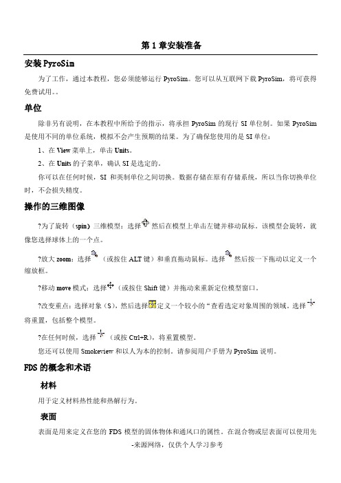
第1章安装准备安装PyroSim为了工作，通过本教程，您必须能够运行PyroSim。

您可以从互联网下载PyroSim，将可获得免费试用。

单位除非另有说明，在本教程中所给予的指示，将承担PyroSim的现行SI单位制。

如果PyroSim 是使用不同的单位系统，模拟不会产生预期的结果。

为了确保您使用的是SI单位：1、在View菜单上，单击Units。

2、在Units的子菜单，确认SI是选定的。

你可以在任何时候，SI和英制单位之间切换。

数据存储在原有存储系统，所以当你切换单位时，不会损失精度。

操作的三维图像?为了旋转（spin）三维模型：选择然后在模型上单击左键并移动鼠标。

该模型会旋转，就像您选择球体上的一个点。

?放大zoom：选择（或按住ALT键）和垂直拖动鼠标。

选择然后按一下拖动以定义一个缩放框。

?移动move模式：选择（或按住Shift键）并拖动来重新定位模型窗口。

?改变重点：选择对象（S），然后选择定义一个较小的“查看选定对象周围的领域。

选择将重置，包括整个模型。

?在任何时候，选择（或按Ctrl+R），将重置模型。

您还可以使用Smokeview和以人为本的控制。

请参阅用户手册为PyroSim说明。

FDS的概念和术语材料用于定义材料热性能和热解行为。

表面表面是用来定义在您的FDS模型的固体物体和通风口的属性。

在混合物或层表面可以使用先前定义的材料。

默认情况下，所有的固体物体和通风口都是有惰性的，一个固定的温度，初始温度。

障碍物障碍物的根本在火灾动力学模拟的几何表示（FDS）[FDS-SMV的官方网站]。

障碍物两点定义在三维的矩形固体空间。

表面特性，被分配到每个面对的阻挠。

设备和控制逻辑可以定义创建或删除在模拟过程中的一个障碍。

当创建一个模型，障碍物的几何形状并不需要相匹配的几何网格的解决方案中使用。

然而，产品安全的解决方案将配合所有几何解决方案网状。

在FDS分析，阻塞所有的面转移到对应最近的网状细胞。

齐齐哈尔大学毕业设计(论文)题目年产6万吨2-丙基庚醇车间合成工段工艺初步设计学院化学与化学工程专业班级学生姓名指导教师成绩2013 年 6 月日摘要本课题是年产6万吨2-丙基庚醇车间合成工段工艺的初步设计。

第一论述了二丙基庚醇合成的意义与作用、国内外研究现状及进展前景，并简要介绍了二丙基庚醇的性质及合成方式，第二介绍了课题的设计背景、厂址选择和原料产品规格；通过国内外几种相关工艺的比较肯定本设计的工艺流程，对整个生产进程进行了物料衡算、热量衡算和Aspen plus模拟；对反映釜等主要设备进行了设备计算与选型，而且对车间设备进行了布置，对自动控制、安全和环境保护和公用工程进行了概述。

最后按照毕业设计的要求利用AutoCAD绘制戊醛缩合反映釜装配图和合成工段设备平立面布置图，手绘了带控制点的工艺流程图，而且完成了20 000字的毕业设计说明书。

关键词：初步设计；合成工段；2-丙基庚醇；衡算AbstractThe preliminary design of workshop of the synthesis section of 60,000 tons annual production capacity of 2-propyl heptanol was completed. Firstly, the significance, the function of 2-propyl heptanol, the development of research on 2-propyl heptanol was stated. The nature of 2-propyl heptanol and synthetic methods were described briefly. Secondly, the design background, plant location and materials and product specification were introduced; comparion of the productive processed in the domestic and aboard, the design process was determined. Meanwhile the material balance, heat balance, and the simulation of process by Aspen plus were finished. The reactor equipment and other major equipments were calculated and selected. And the layout of the equipment for the workshop, safety, environmental protection and public works were outlined. Thirdly, the equipments arrangement diagram of the workshop and the pentanal condensation reactor equipment were drawn with Auto CAD, the process flow diagram with control points was drawn by hand. Finally, the design instruction of 20 thousand words was finished.Key words：Preliminary design; Synthesis section; 2 - propyl heptanol; Balance calculation目录摘要 (I)Abstract (II)第一章总论 (1)概述 (1)项目建设意义 (1)国内外现状及进展前景 (1)设计依据 (3)厂址选择 (4)厂址肯定 (4)厂址优势分析 (4)设计规模与生产制度 (5)设计规模 (5)生产制度 (5)原料和产品规格 (6)经济核算 (6)第2章工艺设计和计算 (7)工艺线路的选择 (7)2-丙基庚醇工艺介绍 (7)2-丙基庚醇工艺的肯定 (8)工艺流程简述 (8)物料衡算 (9)反映器R101的物料衡算 (9)分离罐V103的物料衡算 (10)换热器E101的物料衡算 (11)精馏塔T101的物料衡算 (12)换热器E104的物料衡算 (12)反映器R102的物料衡算 (13)换热器E105的物料衡算 (14)闪蒸罐V105的物料衡算 (15)热量衡算 (16)反映器R101的热量衡算 (16)换热器E101的热量衡算 (17)T101冷凝器E102的热量衡算 (18)T101再沸器E103的热量衡算 (19)精馏塔T101的热量衡算 (21)换热器E104的热量衡算 (22)反映器R102的热量衡算 (24)换热器E105的热量衡算 (25)全流程模拟 (26)总工艺的模拟 (26)反映器R101的模拟 (27)精馏塔T101的模拟 (28)反映器R102的模拟 (28)第3章设备计算及选型 (30)关键设备R101计算及选型 (30)R101筒体直径和高度的计算 (30)筒体壁厚的计算 (30)夹套的计算 (31)水压实验及强度校核 (32)换热计算 (33)釜体法兰的选择 (33)搅拌器的选择 (33)搅拌传动装置和密封装置的选择 (34)容器支座的选择 (35)人孔、视镜、温度计和工艺接管的选择 (35)其他设备计算与选型 (36)反映器R102的计算 (36)精馏塔T101的计算 (37)换热器的计算与选型 (40)泵计算与选型 (43)储罐和回流罐的计算与选型 (44)紧缩机C101的计算与选型 (46)第4章设备一览表 (47)第5章车间布置 (49)反映器和塔的布置 (49)换热器的布置 (50)泵和紧缩机的布置 (50)罐的布置 (51)第6章自动控制 (52)2-丙基庚醇合成工段自动控制 (52)泵P101的控制 (52)塔顶冷凝器E102的控制 (52)反映器R101的控制 (53)精馏塔T101的控制 (53)第7章公用工程 (55)供水 (55)供热 (55)供电 (56)第8章安全环境保护 (57)结束语 (58)参考文献 (59)致谢 (61)第一章总论概述项目建设意义分子总碳数为4～13的脂肪族伯醇，其全世界近50％产量用于生产增塑剂，所以国内外俗称其为增塑剂醇[1]。

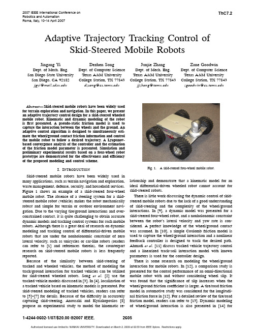
Trans. Nonferrous Met. Soc. China 22(2012) 1064í1072Correlation between welding and hardening parameters offriction stir welded joints of 2017 aluminum alloyHassen BOUZAIENE, Mohamed-Ali REZGUI, Mahfoudh AYADI, Ali ZGHALResearch Unit in Solid Mechanics, Structures and Technological Development (99-UR11-46),Higher School of Sciences and Techniques of Tunis, TunisiaReceived 7 September 2011; accepted 1 January 2011Abstract: An experimental study was undertaken to express the hardening Swift law according to friction stir welding (FSW) aluminum alloy 2017. Tensile tests of welded joints were run in accordance with face centered composite design. Two types of identified models based on least square method and response surface method were used to assess the contribution of FSW independent factors on the hardening parameters. These models were introduced into finite-element code “Abaqus” to simulate tensile tests of welded joints. The relative average deviation criterion, between the experimental data and the numerical simulations of tension-elongation of tensile tests, shows good agreement between the experimental results and the predicted hardening models. These results can be used to perform multi-criteria optimization for carrying out specific welds or conducting numerical simulation of plastic deformation of forming process of FSW parts such as hydroforming, bending and forging.Key words: friction stir welding; response surface methodology; face centered central composite design; hardening; simulation; relative average deviation criterion1 IntroductionFriction stir welding (FSW) is initially invented and patented at the Welding Institute, Cambridge, United Kingdom (TWI) in 1991 [1] to improve welded joint quality of aluminum alloys. FSW is a solid state joining process which was therefore developed systematically for material difficult to weld and then extended to dissimilar material welding [2], and underwater welding [3]. It is a continuous and autogenously process. It makes use of a rotating tool pin moving along the joint interface and a tool shoulder applying a severe plastic deformation [4].The process is completely mechanical, therefore welding operation and weld energy are accurately controlled. B asing on the same welding parameters, welding joint quality is similar from a weld to another.Approximate models show that FSW could be successfully modeled as a forging and extrusion process [5]. The plastic deformation field in FSW is compared with that in metal cutting [6í8]. The predominant deformation during FSW, particularly in vicinities of thetool, is expected to be simple shear, and parallel to the tool surface [9]. When the workpiece material sticks to the tool, heat is generated at the tool/workpiece contact due to shear deformation. The material becomes in paste state favoring the stirring process within the thermomechanically affected zone, causing a large plastic deformation which alters micro and macro structure and changes properties in polycrystalline materials [10].The development of the mechanical behavior model, of heterogeneous structure of the welded zone, is based on a composite material approach, therefore it must takes into account material properties associated with the different welded regions [11]. The global mechanical behavior of FSW joint was studied through the measurement of stress strain performed in transverse [12,13] and longitudinal [14] directions compared with the weld direction. Finite element models were also developed to study the flow patterns and the residual stresses in FSW [15]. B ased on all these models, numerical simulations were performed in order to investigate the effects of welding parameters and tool geometry on welded material behaviors [16] to predict the feasibility of the process on various shape parts [17].Corresponding author: Mohamed-Ali REZGUI; E-mail: mohamedali.rezgui@ DOI: 10.1016/S1003-6326(11)61284-3Hassen BOUZAIENE, et al/Trans. Nonferrous Met. Soc. China 22(2012) 1064í1072 1065 However, the majority of optimization studies of theFSW process were carried out without being connectedto FSW parameters.In the present study, from experimental andmodeling standpoint, the mechanical behavior of FSWaluminum alloy 2017 was examined by performingtensile tests in longitudinal direction compared with theweld direction. It is a matter of identifying the materialparameters of Swift hardening law [18] according to theFSW parameters, so mechanical properties could bepredicted and optimized under FSW operating conditions.The strategy carried out rests on the response surfacemethod (RSM) involving a face centered centralcomposite design to fit an empirical models of materialparameters of Swift hardening law. RSM is a collectionof mathematical and statistical technique, useful formodeling and analysis problems in which response ofinterest is influenced by several variables; its objective isto optimize this response [19]. The diagnostic checkingtests provided by the analysis of variance (ANOV A) suchas sequential F-test, Lack-of-Fit (LoF) test, coefficient ofdetermination (R2), adjusted coefficient of determination(2adjR) are used to select the adequacy models [20].2 Experimental2.1 Welding processThe aluminum alloy 2017 chosen for investigationhas good mechanical characteristics (Table 1), excellentmachinability and formability, and is mostly used ingeneral mechanics applications from high strengthsuitable for heavy-duty structural parts.Table 1 Mechanical properties of aluminum alloy 2017Ultimate tensile strength/MPaYieldstrength/MPaElongation/%Vickershardness427 276 22 118 The experimental set up used in this study was designed in Kef Institute of Technology (Tunisia). A 7.5 kW powered universal mill (Momac model) with 5 to 1700 r/min and welding feed rate ranging from 16 to 1080 mm/min was used. Aluminum alloy 2017 plate of6 mm in thickness was cut and machined into rectangular welding samples of 250 mm×90 mm. Welding test was performed using two samples in butt-configuration, in contact along their larger edge, fixed on a metal frame which was clamped on the machine milling table.To ensure the repeatability of the FSW process, clamping torque and flatness surface of the plates to be welded are controlled for each welding test. At the end of welding operation, around 80 s are respected before the withdrawal of the tool and the extracting of the welded parts. In this experimental study, we purpose to screen theeffects of three operating factors, i.e. tool rotational speed N, tool welding feed F and diameter ratio r, on hardening parameters from Swift’s hardening law such as strength coefficient (k), initial yield strain (İ0) and hardening exponent (n). The ratio (r=d/D) of pin diameter (d) to shoulder diameter (D), is intended to optimize the tool geometry [21í23]. The welding tool is manufactured from a high alloy steel (Fig. 1).Fig. 1 FSW tool geometry (mm)Preliminary welding tests were performed to identify both higher and lower levels of each considered factors. These limits are fixed from visual inspections of the external morphology and cross sections of the welded joints with no macroscopic defects such as surface irregularities, excessive flash, and lack of penetration or surface-open tunnels. However, among these limits one is not sure to have a safe welded joint so often, but they show great potential on defect avoidance. Figure 2 shows some external macroscopic defects observed beyond the limit levels established for each factor. Table 2 lists the processing factors as well as levels assigned to each, and Table 3 shows the fixed levels for other factors needed to success the welding tests.A face centered central composite design, which comes under the RSM approach, with three factors was used to characterize the nature of the welded joints by determining hardening parameters. In this design the star points are at the center of each face of the factorial space (Į=±1), all factors are run at three levels, which are í1, 0, +1 in term of the coded values (Table 4). The experiment plan has been run in random way to avoid systematic errors.2.2 Tensile testsThe tensile tests are performed on a Testometric’s universal testing machines FSí300 kN. The tensile test specimens (ASME E8Mí04) proposed for characterizing the mechanical behavior of the FSW joint, were cut inHassen BOUZAIENE, et al/Trans. Nonferrous Met. Soc. China 22(2012) 1064í10721066Fig. 2 Types of macroscopic defectsTable 2 Levels for operating parameters for FSW processFactorLow level (í1) Center point (0) High level(+1)N /(r·min í1) 653 910 1280 F /(mm·min í1)67 86 109r /%33 39 44Table 3 Welding parametersPin height/ mm Shoulder diameter/ mm Small diameter pin/mm Tool’s inclination angle/(°) Penetrationdepth of shoulder/mm5.3 18 4 30.78longitudinal direction compared with the weld direction, so that active zone is enclosed in the central weld zone (Fig. 3). Figure 4 shows the tensile specimens after fracture.Ultimately, it is a matter of experimental evaluation of hardening parameters of the behavior of FSW joints (k , İ0, n ) according to Swift’s hardening law:n k )(p 0H H V (1)These parameters are required to identify the plastic deformation aptitude of the FSW joints. They are also needed for numerical simulations of forming operations on welded plates. The hardening parameters have been calculated by least square method (LSM) from the stressüstrain curves data. Table 4 shows the experimental design as well as dataset performance characteristics according to the FSW parameters of aluminum Alloy 2017.3 Experimental results3.1 Development of mathematical modelsAlthough the basic principles of FSW are very simple, it involves complex phenomena related to thermo-mechanical and metallurgical transformation that causes strong microstructural heterogeneities in the welded zone. From an energy standpoint, welding process is generated by converting mechanical energy provided by FSW tool into other types of energy such as heat, plastic deformation and microstructural transformations. The nonlinear character of these different dissipation forms can justify research for nonlinear prediction models whose accuracy generally depends on the order of the models relating the responses to welding parameters. For this reason, we chose the RSM which is helpful in developing a suitable approximation for the true functional relationships between quantitative factors (x 1, x 2, Ă, x k ) and the response surface or response functions Y (k , İ0, n ) that may characterize the nature of the welded joints as follows:r 21),,,(e x x x f Y k (2)Hassen BOUZAIENE, et al/Trans. Nonferrous Met. Soc. China 22(2012) 1064í10721067Table 4 Face centered central composite design for FSW of aluminum alloy 2017Factors levelCoded Actual Hardening parameterTypeStandard orderN F r N /(r·m í1)F /(mm·min í1)r /% k /MPan İ0/%1 í1 í1 í165367 33629.7 0.3296 0.00202 1 í1 í1 1280 67 33 654.7 0.4514 0.0035 3 í1 1 í1 653109 33 587.8 0.3712 0.0025 4 1 1 í1 1280 109 33 689.2 0.4856 0.00555 í1 í1 1 653 67 44 642.3 0.4524 0.00256 1 í1 1128067 44 218.6 0.2447 0.0015 7 í1 1 1 653 109 44 685.5 0.4885 0.0035 Factorialdesign8 1 1 1 1280 109 44 332.5 0.3405 0.00209 0 0 0 91086 39 624.9 0.4257 0.0025 10 0 0 0 910 86 39 639.9 0.4292 0.0025 11 0 0 0 910 86 39 640.9 0.4011 0.0020 Center point12 0 0 0 910 86 39 598.6 0.3960 0.0023 13 í1 0 0 653 86 39 690.6 0.4748 0.0027 14 1 0 0 128086 39 505.6 0.3909 0.0030 15 0 í1 091067 39499 0.3317 0.001716 0 1 0 910 109 39 545.6 0.4157 0.0026 17 0 0 í1 910 86 33 672.1 0.4385 0.0027 Star point18 0 019108644 509.7 0.41750.0019Fig. 3 Tensile test specimens (ASME E8Mí04) cut in longitudinal direction compared with weld direction (mm)Fig. 4 Tensile specimens after fractureThe residual error term (e r ) measures theexperimental errors. Such relationship was developed as quadratic polynomial under multiple regression form [19,20]:¦¦¦ r 20e x x b x b x b b Y j i ij i ii i i (3)where b 0 is an intercept or the average of response; b i , b ii , and b ij represent regression coefficients. For the three factors, the selected polynomial could be expressed as:2332222113210r b F b N b r b F b N b b YFr b Nr b NF b 231312 (4)In applying the RSM, the independent variable Y was viewed as surface to which a mathematical model was fitted. The adequacy of the developed model was tested using the analysis of variance (ANOV A) which quantifies the amount of variation in a process and determines if it is significant or is caused by random noise.3.2 Mathematic model of hardening parametersTable 5 lists the coefficients of the best linear regression models. All selected parameters (N , F , r ) for k and İ0 are statistically significant (P-value less than 0.05) at the 95% confidence level. However, for the response n , the term b 3r having a P-value=0.0654>0.05 is not statistically significant at the 95% confidence level even though the term b 13Nr is statistically significant. Consequently, b 3(r ) is kept in the model to improve the Lack-of-Fit test (Table 6). Furthermore, only theHassen BOUZAIENE, et al/Trans. Nonferrous Met. Soc. China 22(2012) 1064í10721068Table 5 Coefficients of regression models for hardening parametersStrength coefficient (k) Hardeningcoefficient(n) Initial yield strain (İ0) CoefficientEst. SEP-value Est SE P-valueEst/10í4 SE/10í4 P-value b0 610.39,48<10í4 0.422 0.0073 <10-4 22.8 1.010 <10-4 b1 í83.58.48<10í4 í0.020 0.0065 0.0091 2.30 0.912 0.0267 b2 19.68.480.0410.0290.00650.00084.900.9120.0002b3 í84.58.48<10í4 í0.013 0.0065 0.0654 í4.80 0.912 0.0002 b11 5.561.3670.0009b22 í61.812.720.0005í0.0310.00980.009b33b12b13 í112.99.48<10í4 í0.074 0.0073 <10-4 -8,75 1.010 <10-4 b23R2 95.90% 92.38% 92.84%2adjR 94.19% 89.21% 89.86% SE of est. 30.7 0.021 2.9×10í4Est: Estimate; SE: Standard Error; SE of est.: Standard error of estimateTable 6 ANOV A for hardening parametersk n İ0Source of variationSS Df P-Value SS Df P-Value SS/10í7 Df P-Value Model 263946.0 5 <10í4 0.062357 5 <10í4 129.324 5 <10í4Residual 11296.4 12 0.005140912 9.97 12Lack-of-Fit 10130.4 9 0.2065 0.00428669 0.3678 8.295 9 0.3723 Pure error 1166.07 3 0.0008543 3 1.675 3 Total correction 275243.017 0.06749817 139.294 17 DW-value 1.31 1.42 2.26DW: Durbin-Watson statistic; SS: Sum of squares; D f: Degree of freedominteraction (Nír) is statistically significant on the three responses (Fig. 5). According to the adjusted R2 statistic, the selected models explain 94.19%, 89.21% and 89.86% of the variability in k, n and İ0 respectively.The ANOV A (Table 6) for the hardening parameter shows that all models (k, n, İ0) represent statistically significant relationships between the variables in each model at the 99% confidence level (P-value<10í4). The Lack-of-Fit test confirms that these models (k, n, İ0) are adequate to describe the observed data (P-value>0.05) at the 95% confidence level. The DW statistic test indicates that there is probably not any serious autocorrelation in their residuals (DW-value>1.4). The normal probability plots of the residuals suggest that the error terms, for these models, are indeed normally distributed (Fig. 6). The response surface models in terms of coded variables (Eqs. (5)í(7)) are shown in Fig. 7.k=610.3–83.5 N+19.6 F–84.5 r –61.8 F2–112.9 Nr(5) n=0.422–0.020 N+0.029 F–0.013 r–0.031 F2–0.074 Nr(6) İ0=22.8+2.3 N+4.90 F–4.80 r+5.56 N2–8.75 Nr(7) Fig. 5 Interaction plots of Nír (rotational speedídiameter ratio): (a) Strength coefficient k; (b) Hardening coefficient n;(c) Initial yield strain İ0Hassen BOUZAIENE, et al/Trans. Nonferrous Met. Soc. China 22(2012) 1064í1072 1069Fig. 6 Normal probability plots for residual: (a) Strength coefficient k; (b) Hardening coefficient n; (c) Initial yield strain İ04 Validation of identified modelsValidation tests of the identified models were performed through comparative study between the experimental models (EM) of tensile tests and the computed responses given by numerical simulations of the same tests (Fig. 8). The computed responses, expressed in the form of tension and elongation, wereFig. 7 Response surfaces plots: (a) Strength coefficient k;(b) Hardening coefficient n; (c) Initial yield strain İ0 established by examining welded joints having an elastoplastic behavior in accordance with the Swift hardening law (Eq. (1)). These computed responses were deduced from the numerical simulations using the finite element code Abaqus/Implicit, in which the introduced elastoplastic behavior was obtained from the least square hardening models (LSHM) (Table 4) and the response surface hardening models (RSHM) (Table 5). The highest deviations (<10%), between EM and computed response, were recorded with the RSHM. Increasing deviations, as shown in Fig. 8, is due to the effect of combining damage with plastic strains accumulatedHassen BOUZAIENE, et al/Trans. Nonferrous Met. Soc. China 22(2012) 1064í10721070Fig. 8 Relationship between tension and elongation: Confrontation between experimental model (EM), and computed responses (LSHM, RSHM) for three experimental testsduring the onset of localized necking.The relative average deviation criterion (EM/LSHM ]) between the experimental data and the numerical predictions of tensions, was used to assess the quality of the identified models.¦¸¸¹·¨¨©§'' '2exp num exp exp/num )()()(1i i i L F L F L F N] (8)where N is the number of experimental measurements,F exp (ǻL i ) and F num (ǻL i ) are respectively the experimental and predicated tensions relating to the i-th elongation ǻL i . Figure 9 illustrates that the relative average deviation of EM/LSHM (EM/LSHM ]) ranges between 1.64% and 6.75% while the relative average deviation of EM/RSHM (EM/RSHM ]) ranges between 4.52% and 9.32%.Fig. 9 Distribution of relative average deviations for most representative experimental testsFor the deviation within limits fluctuating between 4.52% and 6.75% the estimated models (LSHM and RSHM) are comparable. This applies particularly to welded joints characterized by a strength coefficient (k ), ranging from 520 to 610 MPa and a hardening exponent (n ) ranging between 0.30 and 0.45.5 DiscussionIn this study we evaluated, using RSM, the effect of FSW parameters such as tool rotational speed, welding feed rate and diameter ratio of pin to shoulder on the plastic deformation aptitudes of welded joints. The performed analysis highlights the incontestable significant effects of rotational speed (N ), welding feed rate (F ) and the interaction (Nír ) between rotational speed and diameters ratio on hardening parameters (k , n , İ0) according to Swift law. The established models show that tool diameter ratio has a linear effect only on (k ) and (İ0), it does not have any quadratic effect. They also show that rotational speed has a quadratic effect solely on (İ0); while welding feed rate has a quadratic effect on both (k ) and (n ).In addition, numerical simulation of tensile tests of welded joints has been made possible through the predictive models (LSHM and RSHM) of Swift’s hardening parameters. To judge whether the models represent correctly the data, a comparative study between the experimental response and the computed response, expressed in terms of tension-elongation, was carried out. It was found that the relative average deviation betweenHassen BOUZAIENE, et al/Trans. Nonferrous Met. Soc. China 22(2012) 1064í1072 1071experimental model and numerical models is less than 9.5% in all cases.Moreover, correlation between welding and hardening parameters provided has many benefits. The correlation relationships can solve inverse problem relating to optimal choice of parameters linked up with the desired welded joints properties to produce welds having tailor-made mechanical properties. The correlation predictions offer the possibility to identify the behavior of friction stir welded joints necessary for finite element simulations of various forming processes while minimizing experimental cost and time. Ultimately, understanding correlations can be useful for studies on reliability of welded assemblies in service life expectancy.6 Conclusions1) Rotational speed and welding feed rate are the factors that have greater influence on hardening parameters (k, n, İ0), followed by diameter ratio that has no influence on the hardening coefficient (n).2) The numerical models RSHM were compared with those through LSHM and confronted to the experimental results. Indeed, within the limit of a relative average deviation of about 9.3%, between the experimental model and numerical models expressed in terms of tension-elongation, the validity of these models is acceptable.3) The predictive models of work-hardening coefficients, established taking into account the FSW parameters, have made possible the numerical simulation of tensile tests of FSW joints. These results can be used to perform multi-criteria optimization for producing welds with specific mechanical properties or conducting numerical simulation of plastic deformation of forming process of friction stir welded parts such as hydroforming, bending and forging.References[1]THOMAS W M, NICHOLAS E D, NEEDHAM J C, MURCH M G,TEMPLE-SMITH P, DAWES C J. Friction stir butt welding,PCT/GB92/ 02203 [P]. 1991.[2]XUE P, NI D R, WANG D, XIAO B L, MA Z Y. Effect of friction stirwelding parameters on the microstructure and mechanical propertiesof the dissimilar AlíCu joints[J]. Materials Science and EngineeringA, 2011, 528: 4683í4689.[3]LIU H J, ZHANG H J, YU L. Effect of welding speed onmicrostructures and mechanical properties of underwater friction stirwelded 2219 aluminum alloy [J]. Materials and Design, 2011, 32:1548í1553.[4]MISHRA R S, MA Z Y. Friction stir welding and processing [J].Materials Science and Engineering R, 2005, 50: 1í78.[5]ARB EGAST W J. A flow-partitioned deformation zone model fordefect formation during friction stir welding [J]. Scripta Materialia,2008, 58: 372í376.[6]LEWIS N P. Metal cutting theory and friction stir welding tooldesign [M]. NASA Faculty Fellowship Program Marshall SpaceFlight Center, University of ALABAMA, NASA/MSFC Directorate:Engineering (ED-33), 2002.[7]ARB EGAST W J. Modeling friction stir welding joining as ametalworking process, hot deformation of aluminum alloys III [C].San Diego: TMS Annual Meeting, 2003: 313í327.[8]ARTHUR C N Jr. Metal flow in friction stir welding [R]. NASAmarshall space flight center, EM30. Huntsville, AL 35812.[9]FONDA R W, B INGERT J F, COLLIGAN K J. Development ofgrain structure during friction stir welding [J]. Scripta Materialia,2004, 51: 243í248.[10]NANDAN R, DEBROY T, BHADESHIA H K D H. Recent advancesin friction stir weldingüProcess, weldment structure and properties[J]. Progress in Materials Science, 2008, 53: 980í1023.[11]LOCKWOOD W D, TOMAZ B, REYNOLDS A P. Mechanicalresponse of friction stir welded AA2024: Experiment and modeling[J]. Materials Science and Engineering A, 2002, 323: 348í353. [12]SALEM H G, REYNOLDS A P, LYONS J S. Microstructure andretention of superplasticity of friction stir welded superplastic 2095sheet [J]. Scripta Materialia, 2002, 46: 337í342.[13]LOCKWOOD W D, REYNOLDS A P. Simulation of the globalresponse of a friction stir weld using local constitutive behavior [J].Materials Science and Engineering A, 2003, 339: 35í42.[14]SUTTON M A, YANG B, REYNOLDS A P, YAN J. B andedmicrostructure in 2024–T351 and 2524-T351 aluminum friction stirwelds, Part II. Mechanical characterization [J]. Materials Science andEngineering A, 2004, 364: 66í74.[15]ZHANG H W, ZHANG Z, CHEN J T. The finite element simulationof the friction stir welding process [J]. Materials Science andEngineering A, 2005, 403: 340í348.[16]ZHANG Z, ZHANG H W. Numerical studies on controlling ofprocess parameters in friction stir welding [J]. Journal of MaterialsProcessing Technology, 2009, 209: 241í270.[17]B UFFA G, FRATINI L, SHIVPURI R. Finite element studies onfriction stir welding processes of tailored blanks [J]. Computers andStructures, 2008, 86: 181í189.[18]SWIFT H W. Plastic instability under plane stress [J]. Journal of theMechanics and Physics of Solids, 1952, 1: 1í18.[19]MONTGOMERY D C. Design and analysis of experiments [M].Fifth Edition. New York: John Wiley & Sons, 2001: 684.[20]MYERS R H, MONTGOMERY D C, ANDERSON-COOK C M.Response surface methodology: Process and product optimizationusing designed experiment [M]. 3rd Edition. New York: John Wiley& Sons, 2009: 680.[21]VIJAY S J, MURUGAN N. Influence of tool pin profile on themetallurgical and mechanical properties of friction stir welded Al–10% TiB2 metal matrix composite [J]. Materials and Design,2010, 31: 3585í3589.[22]ELANGOV AN K, BALASUBRAMANIAN V. Influences of tool pinprofile and tool shoulder diameter on the formation of friction stirprocessing zone in AA6061 aluminum alloy [J]. Materials andDesign, 2008, 29: 362í373.[23]PALANIVEL R, KOSHY MATHEWS P, MURUGAN N.Development of mathematical model to predict the mechanicalproperties of friction stir welded AA6351 aluminum alloy [J]. Journalof Engineering Science and Technology Review, 2011, 4(1): 25í31.Hassen BOUZAIENE, et al/Trans. Nonferrous Met. Soc. China 22(2012) 1064í107210722017䪱 䞥 ⛞ ⛞⹀ ⱘ ㋏Hassen BOUZAIENE, Mohamed-Ali REZGUI, Mahfoudh AYADI, Ali ZGHALBesearch Unit in Solid Mechanics, Structures and Technological Development (99-UR11-46),Higher School of Sciences and Techniques of Tunis, Tunisia㽕˖ 2017䪱 䞥䖯㸠 ⛞ ˈ㸼䗄Swift⹀ 㾘 DŽ䞛⫼䴶 䆒䅵 ⊩䖯㸠⛞ ⱘ Ԍ 偠䆒䅵DŽ䞛⫼ Ѣ ѠЬ⊩ 䴶⊩ⱘ2⾡῵ 䆘Ԅ ⛞ ⛞ ㋴ ⹀ ⱘ DŽ䞛⫼ 䰤 ⿟ Abaqus ῵ ⛞ Ԍ⌟䆩㒧 DŽⳌ 㒧 㸼 ˈ 偠㒧 ῵ 㒧 䕗 DŽ䖭ѯ㒧 㛑⫼Ѣ 偠 Ⳃ Ӭ ˈ 㸠 ԧ⛞ ⛞ 䳊ӊ 䖛⿟Ё ⱘ ῵ ˈ ⎆ ǃ 䬏䗴DŽ䬂䆡˖ ⛞ ˗ 䴶 ⊩˗䴶 Ё 䆒䅵˗⹀ ˗῵ ˗Ⳍ(Edited b y LI Xiang-qun)。

化工进展Chemical Industry and Engineering Progress2023 年第 42 卷第 S1 期基于动力学分析的核桃壳最佳炭化工艺刘阳，王云刚，修浩然，邹立，白彦渊（西安交通大学热流科学与工程教育部重点实验室，陕西 西安 710049）摘要：核桃壳产量多，固定碳含量极高且灰分少。

选取核桃壳作为研究对象，对其炭化过程的热动力学参数进行分析，探究其炭化进程及原理，最终通过实验和响应面模拟分析得到核桃壳炭化的最佳工艺。

研究发现，综合炭化特性指数随着升温速率的增大呈先增大后减小的趋势，且在10℃/min 左右时指数达到峰值，此升温速率下炭化反应更剧烈。

核桃壳的炭化过程是一个多阶段的复杂反应过程，其分阶段进行半纤维素、纤维素和木质素的分解，该过程活化能总体逐渐升高。

最后通过模拟和实验分析得出最佳工况为：升温时间为14.8min ，最终温度为324.7℃，保温时间为60min ，材料粒径为5mm 左右，最佳炭保留率为69.4%。

关键词：炭化；动力学分析；响应面分析；最佳炭化工况；农林废弃物中图分类号：X705 文献标志码：A 文章编号：1000-6613（2023）S1-0094-10Optimal carbonization process of walnut shell based on dynamic analysisLIU Yang ，WANG Yungang ，XIU Haoran ，ZOU Li ，BAI Yanyuan(Key Laboratory of Thermo-Fluid Science and Engineering (Ministry of Education), Xi an Jiaotong University, Xi an710049, Shaanxi, China)Abstract: Walnut shell has high yield, high fixed carbon content and low ash content. In this paper, the walnut shell was selected as the research object, the comprehensive pyrolysis characteristic index was proposed, the thermal dynamics analysis was carried out on it, and the carbonization process and principle were studied. Finally, the best carbonization process was obtained through experiments and response surface simulation analysis. It was found that the comprehensive characteristic index of pyrolysis first increased and then decreased with the increase of heating rate, and reached the peak at about 10℃/min since the pyrolysis reaction was more intense at this heating rate. The carbonization process of walnut shell was a multi-stage complex reaction process, which decomposed hemicellulose, cellulose and lignin in stages, and the activation energy of this process increased gradually. Finally, through simulation and experimental analysis, the optimal process was obtained as follows: heating time was 14.8min, final temperature was 324.7℃, soaking time was 60min, material particle size was about 5 mm and the optimal carbonization rate was 69.4%.Keywords: carbonization; dynamic analysis; response surface analysis; optimal carbonization condition;agricultural and forestry waste研究开发DOI ：10.16085/j.issn.1000-6613.2023-0809收稿日期：2023-05-15；修改稿日期：2023-06-21。

Elsevier期刊被SCI收录最新一期题录信息本内容包括：主题、各主题有代表性刊名、该刊最新一期目录信息（包括卷期、论文题名、页码及作者等）Automation & Control Systems（自动化及控制系统）SYSTEMS & CONTROL LETTERSVolume 59, Issue 5, Pages 265-322 (May 2010)1.Editorial BoardPage IFC2.Gain-scheduled open-loop system design for LPV systems using polynomially parameter-dependent Lyapunov functionsPages 265-276Masayuki Sato3.Delay-adaptive feedback for linear feedforward systemsPages 277-283Nikolaos Bekiaris-Liberis, Miroslav Krstic4.Implicit Euler numerical scheme and chattering-free implementation of sliding mode systemsPages 284-293Vincent Acary, Bernard Brogliato5.Decentralized dynamic nonlinear controllers to minimize transmit power in cellular networks, Part IPages 294-298Vishwesh V. Kulkarni, Mayuresh V. Kothare, Michael G. Safonov6. ISDS small-gain theorem and construction of ISDS Lyapunov functions for interconnected systemsPages 299-304Sergey Dashkovskiy, Lars Naujok7.An observer for a class of nonlinear systems with time varying observation delay Pages 305-312F. Cacace, A. Germani, C. Manes8.Rendezvous of multiple mobile agents with preserved network connectivity Pages 313-322Housheng Su, Xiaofan Wang, Guanrong ChenBiology（生物学）BIOELECTROCHEMISTRYVolume 79, Issue 1, Pages 1-152 (August 2010)1. Editorial BoardPage IFC2. ContentsPages v-vi3.Electrochemistry of norepinephrine on carbon-coated nickel magnetic nanoparticlesmodified electrode and analytical applicationsPages 1-5Chunli Bian, Qingxiang Zeng, Huayu Xiong, Xiuhua Zhang, Shengfu Wang4.Interaction of surface-attached haemoglobin with hydrophobic anions monitored by on-line acoustic wave detectorPages 6-10Jonathan S. Ellis, Steven Q. Xu, Xiaomeng Wang, Grégoi re Herzog, Damien W.M. Arrigan, Michael Thompson5.Electrochemical impedance spectroscopy of polypyrrole based electrochemical immunosensorPages 11-16A. Ramanavicius, A. Finkelsteinas, H. Cesiulis, A. Ramanaviciene6.Electrochemical and AFM characterization on gold and carbon electrodes of a high redox potential laccase from Fusarium proliferatumPages 17-24K. González Arzola, Y. Gimeno, M.C. Arévalo, M.A. Falcón, A. Hernández Creus7.Improvements in the extraction of cell electric properties from their electrorotation spectrumPages 25-30Damien Voyer, Marie Frénéa-Robin, Franois Buret, Laurent Nicolas8.Electrochemical DNA biosensor for the detection of specific gene related to Trichoderma harzianum speciesPages 31-36Shafiquzzaman Siddiquee, Nor Azah Yusof, Abu Bakar Salleh, Fatimah Abu Bakar, Lee Yook Heng9.Development of electrochemical DNA biosensor based on gold nanoparticle modified electrode by electroless depositionPages 37-42Shufeng Liu, Jing Liu, Li Wang, Feng Zhao10.Herbicides affect fluorescence and electron transfer activity of spinach chloroplasts, thylakoid membranes and isolated Photosystem IIPages 43-49Andrea Ventrella, Lucia Catucci, Angela Agostiano11.Nanostructured polypyrrole-coated anode for sun-powered microbial fuel cells Pages 50-56Yongjin Zou, John Pisciotta, Ilia V. Baskakov12.Anodic oxidation of 3,4-dihydroxyphenylacetic acid on carbon electrodes in acetic acid solutionsPages 57-65Slawomir Michalkiewicz, Agata Skorupa13.A voltammetric Rhodotorula mucilaginosa modified microbial biosensor for Cu(II) determinationPages 66-70Meral Yüce, Hasan Nazır, Gönül Dönmez14.Explore various co-substrates for simultaneous electricity generation and Congo red degradation in air-cathode single-chamber microbial fuel cellPages 71-76Yunqing Cao, Yongyou Hu, Jian Sun, Bin Hou15.Electrochemical oxidation of amphetamine-like drugs and application to electroanalysis of ecstasy in human serumPages 77-83E.M.P.J. Garrido, J.M.P.J. Garrido, N. Milhazes,F. Borges, A.M. Oliveira-Brett16.A l-cysteine sensor based on Pt nanoparticles/poly(o-aminophenol) film on glassy carbon electrodePages 84-89Li-Ping Liu, Zhao-Jing Yin, Zhou-Sheng Yang17.The effects of the electro-photodynamic in vitro treatment on human lung adenocarcinoma cellsPages 90-94Jolanta Saczko, Mariola Nowak, Nina Skolucka, Julita Kulbacka, Malgorzata Kotulska 18.Gadolinium blocks membrane permeabilization induced by nanosecond electric pulses and reduces cell deathPages 95-100Franck M. André, Mikhail A. Rassokhin, Angela M. Bowman, Andrei G. Pakhomov19.Scanning electrochemical microscopy activity mapping of electrodes modified with laccase encapsulated in sol–gel processed matrixPages 101-107Wojciech Nogala, Katarzyna Szot, Malte Burchardt, Martin Jönsson-Niedziolka, Jerzy Rogalski, Gunther Wittstock, Marcin Opallo20.Maltose biosensing based on co-immobilization of α-glucosidase and pyranose oxidasePages 108-113Dilek Odaci, Azmi Telefoncu, Suna Timur21.Plasma membrane permeabilization by trains of ultrashort electric pulses Pages 114-121Bennett L. Ibey, Dustin G. Mixon, Jason A. Payne, Angela Bowman, Karl Sickendick, Gerald J. Wilmink, W. Patrick Roach, Andrei G. Pakhomov22.Effect of nano-topographical features of Ti/TiO2 electrode surface on cell response and electrochemical stability in artificial salivaPages 122-129I. Demetrescu, C. Pirvu, V. Mitran23.Efficiency of the delivery of small charged molecules into cells in vitro Pages 130-135M.S. Venslauskas, S. Šatkauskas, R. Rodaitė-Riševičienė24.Carbon nanotube-enhanced cell electropermeabilisationPages 136-141Vittoria Raffa, Gianni Ciofani, Orazio Vittorio, Virginia Pensabene, Alfred Cuschieri25.Dependence of catalytic activity and long-term stability of enzyme hydrogel films on curing timePages 142-146Joshua Lehr, Bryce E. Williamson, Frédéric Barrière, Alison J. Downard26.Enzymatic flow injection method for rapid determination of choline in urine with electrochemiluminescence detectionPages 147-151Jiye Jin, Masahiro Muroga, Fumiki Takahashi, Toshio NakamuraChemistry Applied（化学应用）CARBOHYDRATE POLYMERSVolume 81, Issue 4, Pages 751-970 (23 July 2010)1.Editorial BoardPage CO22.Adsorption separation of Ni(II) ions by dialdehyde o-phenylenediamine starch from aqueous solutionPages 751-757Ping Zhao, Jian Jiang, Feng-wei Zhang, Wen-feng Zhao, Jun-tao Liu, Rong Li3.Rheological and morphological characterization of the culture broth during exopolysaccharide production by Enterobacter sp.Pages 758-764Vítor D. Alves, Filomena Freitas, Cristiana A.V. Torres, Madalena Cruz, Rodol fo Marques, Christian Grandfils, M.P. Gonçalves, Rui Oliveira, Maria A.M. Reis4.Synthesis and evaluation of N-succinyl-chitosan nanoparticles toward local hydroxycamptothecin deliveryPages 765-768Zhenqing Hou, Jing Han, Chuanming Zhan, Chunxiao Zhou, Quan Hu, Qiqing Zhang5.Synthesis and application of new sizing and finishing additives based on carboxymethyl cellulosePages 769-774Z. El-Sayed Mohamed, A. Amr, Dierk Knittel, Eckhard Schollmeyer6.Synthesis and thermo-physical properties of chitosan/poly(dl-lactide-co-glycolide) composites prepared by thermally induced phase separationPages 775-783Santos Adriana Martel-Estrada, Carlos Alberto Martínez-Pérez, José Guadalupe Chacón-Nava, Perla Elvia García-Casillas, Imelda Olivas-Armendarizparison of the immunological activities of arabinoxylans from wheat bran with alkali and xylanase-aided extractionPages 784-789Sumei Zhou, Xiuzhen Liu, Yan Guo, Qiang Wang, Daiyin Peng, Li Cao8.Nano-in-micro alginate based hybrid particlesPages 790-798Abhijeet Joshi, R. Keerthiprasad, Rahul Dev Jayant, Rohit Srivastava9.The effects of reaction conditions on block copolymerization of chitosan and poly(ethylene glycol)Pages 799-804F. Ganji, M.J. Abdekhodaie10.Thermal behaviour and interactions of cassava starch filled with glycerolplasticized polyvinyl alcohol blendsPages 805-810W.A.W.A. Rahman, Lee Tin Sin, A.R. Rahmat, A.A. Samad11.Banana fibers and microfibrils as lignocellulosic reinforcements in polymer compositesPages 811-819Maha M. Ibrahim, Alain Dufresne, Waleed K. El-Zawawy, Foster A. Agblevor12.Variability of biomass chemical composition and rapid analysis using FT-NIR techniquesPages 820-829Lu Liu, X. Philip Ye, Alvin R. Womac, Shahab Sokhansanj13.TEMPO oxidation of gelatinized potato starch results in acid resistant blocks of glucuronic acid moietiesPages 830-838Ruud ter Haar, Johan W. Timmermans, Ted M. Slaghek, Francisca E.M. Van Dongen, HenkA. Schols, Harry Gruppen14.Development of films based on quinoa (Chenopodium quinoa, Willdenow) starch Pages 839-848Patricia C. Araujo-Farro, G. Podadera, Paulo J.A. Sobral, Florencia C. Menegalli 15.Polysaccharide determination in protein/polysaccharide mixtures for phase-diagram constructionPages 849-854Jacob K. Agbenorhevi, Vassilis Kontogiorgos16.Calorimetric and light scattering study of interactions and macromolecular properties of native and hydrophobically modified hyaluronanPages 855-863Martin Chytil, Sabina Strand, Bjørn E. Christensen, Miloslav Pekař17.Spray drying of nopal mucilage (Opuntia ficus-indica): Effects on powder properties and characterizationPages 864-870F.M. León-Martínez, L.L. Méndez-Lagunas, J. Rodríguez-Ramírez18.Preparation and evaluation of nanoparticles of gum cordia, an anionic polysaccharide for ophthalmic deliveryPages 871-877Monika Yadav, Munish Ahuja19.Functional modification of agarose: A facile synthesis of a fluorescent agarose–guanine derivativePages 878-884Mihir D. Oza, Ramavatar Meena, Kamalesh Prasad, P. Paul, A.K. Siddhanta20.Characterization of maize amylose-extender (ae) mutant starches. Part III: Structures and properties of the Naegeli dextrinsPages 885-891Hongxin Jiang, Sathaporn Srichuwong, Mark Campbell, Jay-lin Jane21.Multistage deacetylation of chitin: Kinetics studyPages 892-896N. Yaghobi, F. Hormozi22.Sulfated modification, characterization and structure–antioxidantrelationships of Artemisia sphaerocephala polysaccharidesPages 897-905Junlong Wang, Hongyun Guo, Ji Zhang, Xiaofang Wang, Baotang Zhao, Jian Yao, Yunpu Wang23.Magnetic chitosan/iron (II, III) oxide nanoparticles prepared by spray-drying Pages 906-910Hsin-Yi Huang, Yeong-Tarng Shieh, Chao-Ming Shih, Yawo-Kuo Twu24.Effect of adding a small amount of high molecular weight polyacrylamide on properties of oxidized cassava starchPages 911-918Yan Liu, Xu-chao Lv, Xiao Hu, Zhi-hua Shan, Pu-xin Zhu25.Preparation of nanofibrillar carbon from chitin nanofibersPages 919-924M. Nogi, F. Kurosaki, H. Yano, M. Takano26.Preparation and characterization of cellulose acetate–Fe2O3 composite nanofibrous materialsPages 925-930Costas Tsioptsias, Kyriaki G. Sakellariou, Ioannis Tsivintzelis, Lambrini Papadopoulou, Costas Panayiotou27.Synthesis, characteristic and antibacterial activity of N,N,N-trimethyl chitosan and its carboxymethyl derivativesPages 931-936Tao Xu, Meihua Xin, Mingchun Li, Huili Huang, Shengquan Zhou28.Fast compositional analysis of ramie using near-infrared spectroscopyPages 937-941Wei Jiang, Guangting Han, Yuanming Zhang, Mengmeng Wang29.Structure characterization of polysaccharide isolated from the fruiting bodies of Tricholoma matsutakePages 942-947Xiang Ding, Su Feng, Mei Cao, Mao-tao Li, Jie Tang, Chun-xiao Guo, Jie Zhang, Qun Sun, Zhi-rong Yang, Jian Zhao30.New insights into viscosity abnormality of sodium alginate aqueous solution Pages 948-952Dan Zhong, Xin Huang, Hu Yang, Rongshi Cheng31.Structural characterization and anti-inflammatory activity of two water-soluble polysaccharides from Bellamya purificataPages 953-960Hong Zhang, Lin Ye, Kuiwu WangComputer Science, Artificial Intelligence（计算机科学，人工智能）ARTIFICIAL INTELLIGENCEVolume 174, Issue 11, Pages 639-766 (July 2010)1.Editorial BoardPage IFC2.Partial observability and learnabilityPages 639-669Loizos Michael3.Monte Carlo tree search in KriegspielPages 670-684Paolo Ciancarini, Gian Piero Favini4.Learning conditional preference networksPages 685-703Frédéric Koriche, Bruno Zanuttini5.Planning to see: A hierarchical approach to planning visual actions on a robot using POMDPsPages 704-725Mohan Sridharan, Jeremy Wyatt, Richard Dearden6.Analysis of a probabilistic model of redundancy in unsupervised information extractionPages 726-748Doug Downey, Oren Etzioni, Stephen Soderland7. Designing competitions between teams of individualsPages 749-766Pingzhong Tang, Yoav Shoham, Fangzhen LinEnergy & Fuels（能源和燃料）APPLIED ENERGYVolume 87, Issue 8, Pages 2427-2768 (August 2010)1.IFCPage IFC2. Energy balance analysis of wind-based pumped hydro storage systems in remote island electrical networksPages 2427-2437J.K. Kaldellis, M. Kapsali, K.A. Kavadias3.Energy auditing and energy conservation potential for glass worksPages 2438-2446Yingjian Li, Jiezhi Li, Qi Qiu, Yafei Xu4.Energy demand and comparison of current defrosting technologies of frozen raw materials in defrosting tunnelsPages 2447-2454Marek Bezovsky, Michal Stricik, Maria Prascakova5.Guidelines for clockspeed acceleration in the US natural gas transmission industry Pages 2455-2466Ruud Weijermars6.Multi-objective self-adaptive algorithm for highly constrained problems: Novel method and applicationsPages 2467-2478Abdelaziz Hammache, Marzouk Benali, François Aubé7.Stochastic interest rates in the analysis of energy investments: Implications on economic performance and sustainabilityPages 2479-2490Athanasios Tolis, Aggelos Doukelis, Ilias Tatsiopoulos8.Effects of the PWM carrier signals synchronization on the DC-link current in back-to-back convertersPages 2491-2499L.G. González, G. Garcerá, E. Figueres, R. González9.Efficiency improvement of the DSSCs by building the carbon black as bridge in photoelectrodePages 2500-2505Chen-Ching Ting, Wei-Shi Chao10.Integer programming with random-boundary intervals for planning municipal power systemsPages 2506-2516M.F. Cao, G.H. Huang, Q.G. Lin11. Modeling the relationship between the oil price and global food prices Pages 2517-2525Sheng-Tung Chen, Hsiao-I Kuo, Chi-Chung Chen12.Marginal production in the Gulf of Mexico – II. Model resultsPages 2526-2534Mark J. Kaiser, Yunke Yu13.Marginal production in the Gulf of Mexico – I. Historical statistics & model frameworkPages 2535-2550Mark J. Kaiser14.Assessment of forest biomass for use as energy. GIS-based analysis of geographical availability and locations of wood-fired power plants in PortugalPages 2551-2560H. Viana, Warren B. Cohen, D. Lopes, J. Aranha15.Alkaline catalyzed biodiesel production from moringa oleifera oil with optimized production parametersPages 2561-2565G. Kafuku, M. Mbarawae of two-component Weibull mixtures in the analysis of wind speed in the Eastern MediterraneanPages 2566-2573S.A. Akdağ, H.S. Bagiorgas, G. Mihalakakou17.Evaluation of wind energy investment interest and electricity generation cost analysis for TurkeyPages 2574-2580Seyit Ahmet Akdağ, Önder Güler18.The role of demand-side management in the grid integration of wind power Pages 2581-2588Pedro S. Moura, Aníbal T. de Almeida19.Synthesis of biodiesel from waste vegetable oil with large amounts of free fatty acids using a carbon-based solid acid catalystPages 2589-2596Qing Shu, Jixian Gao, Zeeshan Nawaz, Yuhui Liao, Dezheng Wang, Jinfu Wang20.A study on the overall efficiency of direct methanol fuel cell by methanol crossover currentPages 2597-2604Sang Hern Seo, Chang Sik Lee21.Study of heat transfer between an over-bed oil burner flame and a fluidized bed during start-up: Determination of the flame to bed convection coefficientPages 2605-2614Vijay Jain, Dominic Groulx, Prabir Basu22.Predictive tools for the estimation of downcomer velocity and vapor capacity factor in fractionatorsPages 2615-2620Alireza Bahadori, Hari B. Vuthaluru23. Monitoring strategies for a combined cycle electric power generatorPages 2621-2627Joshua Finn, John Wagner, Hany Bassily24. Combustion and heat transfer at meso-scale with thermal recuperationPages 2628-2639V. Vijayan, A.K. Gupta25.Part-load characteristics of direct injection spark ignition engine using exhaust gas trapPages 2640-2646Yun-long Bai, Zhi Wang, Jian-xin Wang26.Gas–liquid absorption reaction between (NH4)2SO3 solution and SO2 for ammonia-based wet flue gas desulfurizationPages 2647-2651Xiang Gao, Honglei Ding, Zhen Du, Zuliang Wu, Mengxiang Fang, Zhongyang Luo, Kefa Cen27. Direct contact PCM–water cold storagePages 2652-2659Viktoria Martin, Bo He, Fredrik Setterwall28. Fatty acid eutectic/polymethyl methacrylate composite as form-stable phase change material for thermal energy storagePages 2660-2665Lijiu Wang, Duo Meng29.Thermal characteristics of shape-stabilized phase change material wallboard with periodical outside temperature wavesPages 2666-2672Guobing Zhou, Yongping Yang, Xin Wang, Jinming Cheng30. Study on a compact silica gel–water adsorption chiller without vacuum valves: Design and experimental studyPages 2673-2681C.J. Chen, R.Z. Wang, Z.Z. Xia, J.K. Kiplagat, Z.S. Lu31. Separation characteristics of clathrate hydrates from a cooling plate forefficient cold energy storagePages 2682-2689Tadafumi Daitoku, Yoshio Utaka32. A flexible numerical model to study an active magnetic refrigerator for near room temperature applicationsPages 2690-2698Ciro Aprea, Angelo Maiorino33. Feasibility study of an ice slurry-cooling coil for HVAC and R systems in a tropical buildingPages 2699-2711Y.H. Yau, S.K. Lee34. Optimum sizing of wind-battery systems incorporating resource uncertainty Pages 2712-2727Anindita Roy, Shireesh B. Kedare, Santanu Bandyopadhyay35. Peak current mode control of three-phase boost rectifiers in discontinuous conduction mode for small wind power generatorsPages 2728-2736O. Carranza, G. Garcerá, E. Figueres, L.G. González36. Experimental flow field characteristics of OFA for large-angle counter flow of fuel-rich jet combustion technologyPages 2737-2745Weidong Fan, Zhengchun Lin, Youyi Li, Mingchuan ZhangEngineering, Electrical & Electronic（电机及电子工程）MICROELECTRONIC ENGINEERINGVolume 87, Issue 9, Pages 1655-1808 (November 2010)1. Inside Front Cover - Editorial BoardPage IFC2 PrefacePage 1655Joel Barnett3.In0.53Ga0.47As(1 0 0) native oxide removal by liquid and gas phase HF/H2O chemistriesPages 1656-1660F.L. Lie, W. Rachmady, A.J. Muscat4.A study of the interaction of gallium arsenide with wet chemical formulations using thermodynamic calculations and spectroscopic ellipsometryPages 1661-1664J. Price, J. Barnett, S. Raghavan, M. Keswani, R. Govindarajan5.The removal of nanoparticles from sub-micron trenches using megasonicsPages 1665-1668Pegah Karimi, Taehoon Kim, Juan Aceros, Jingoo Park, Ahmed A. Busnaina6.In-line control of Si loss after post ion implantation stripPages 1669-1673D. Shamiryan, D. Radisic, W. Boullart7.Removal of post-etch 193 nm photoresist in porous low-k dielectric patterning using UV irradiation and ozonated waterPages 1674-1679E. Kesters, Q.T. Le, M. Lux, L. Prager, G. Vereecke8.Repair of plasma-damaged p-SiOCH dielectric films in supercritical CO2Pages 1680-1684Jae Mok Jung, Hong Seok Kwon, Won-Ki Lee, Byung-Chun Choi, Hyun Gyu Kim, Kwon Taek Lim9.Development of compatible wet-clean stripper for integration of CoWP metal cap in Cu/low-k interconnectsPages 1685-1688Aiping Wu, Eugene Baryschpolec, Madhukar Rao, Matthias Schaller, Christin Bartsch, Susanne Leppack, Andreas Ott10.Dissolution and electrochemical impedance spectroscopy studies of thin copper oxide films on copper in semi-aqueous fluoride solutionsPages 1689-1695N. Venkataraman, S. Raghavan11.The sacrificial oxide etching of poly-Si cantilevers having high aspect ratios using supercritical CO2Pages 1696-1700Ha Soo Hwang, Jae Hyun Bae, Jae Mok Jung, Kwon Taek Lim12.Monitoring wafer cleanliness and metal contamination via VPD ICP-MS: Case studies for next generation requirementsPages 1701-1705Meredith Beebe, Scott Anderson13.Fabrication of a two-step Ni stamp for blind via hole application on PWB Pages 1707-1710In-Soo Park, Jin-Soo Kim, Seong-Hun Na, Seung-Kyu Lim, Young-Soo Oh, Su-Jeong Suh 14.Arrays of metallic nanocones fabricated by UV-nanoimprint lithographyPages 1711-1715Juha M. Kontio, Janne Simonen, Juha Tommila, Markus Pessa15.Synthesis, characterization of CeO2@SiO2 nanoparticles and their oxide CMP behaviorPages 1716-1720Xiaobing Zhao, Renwei Long, Yang Chen, Zhigang Chen16.Development of a triangular-plate MEMS tunable capacitor with linear capacitance–voltage responsePages 1721-1727M. Shavezipur, S.M. Hashemi, P. Nieva, A. Khajepour17.The correlation of the electrical properties with electron irradiation and constant voltage stress for MIS devices based on high-k double layer (HfTiSiO:N and HfTiO:N) dielectricsPages 1728-1734V. Mikhelashvili, P. Thangadurai, W.D. Kaplan, G. Eisenstein18. Intra-level voltage ramping-up to dielectric breakdown failure on Cu/porous low-k interconnections in 45 nm ULSI generationPages 1735-1740C.H. Huang, N.F. Wang, Y.Z. Tsai, C.I. Hung, M.P. Houng19. Anodic bonding of glass–ceramics to stainless steel coated with intermediate SiO2 layerPages 1741-1746Dehua Xiong, Jinshu Cheng, Hong Li, Wei Deng, Kai Ye20.Preparation of silica/ceria nano composite abrasive and its CMP behavior on hard disk substratePages 1747-1750Hong Lei, Fengling Chu, Baoqi Xiao, Xifu Tu, Hua Xu, Haineng Qiu21.Investigation on the controllable growth of monodisperse silica colloid abrasives for the chemical mechanical polishing applicationPages 1751-1755XiaoKai Hu, Zhitang Song, Haibo Wang, Weili Liu, Zefang Zhang22.Fabrication and electrical characteristics of ultrathin (HfO2)x(SiO2)1−x films by surface sol–gel method and reaction-anneal treatmentPages 1756-1759You-Pin Gong, Ai-Dong Li, Chao Zhao, Yi-Dong Xia, Di Wu23.Frequency properties of on-die power distribution network in VLSI circuits Pages 1760-1763Pavel Livshits, Yefim Fefer, Anton Rozen, Yoram Shapira24.Analytical modelling for the current–voltage characteristics of undoped or lightly-doped symmetric double-gate MOSFETsPages 1764-1768A. Tsormpatzoglou, D.H. Tassis, C.A. Dimitriadis, G. Ghibaudo, G. Pananakakis, N. Collaert25.Anti-buckling S-shaped vertical microprobes with branch springsPages 1769-1776Jung Yup Kim, Hak Joo Lee, Young-Ho Cho26.Characterization of UV photodetectors with MgxZn1−xO thin filmsPages 1777-1780Tung-Te Chu, Huilin Jiang, Liang-Wen Ji, Te-Hua Fang, Wei-Shun Shi, Tian-Long Chang, Teen-Hang Meen, Jingchang Zhong27.Barrier height temperature coefficient in ideal Ti/n-GaAs Schottky contacts Pages 1781-1784T. Göksu, N. Yıldırım, H. Korkut, A.F. Özdemir, A. Turut, A. Kökçe28.Optical coherence tomography for non-destructive investigation of silicon integrated-circuitsPages 1785-1791K.A. Serrels, M.K. Renner, D.T. Reid29.Materials selection procedure for RF-MEMSPages 1792-1795G. Guisbiers, E. Herth, B. Legrand, N. Rolland, T. Lasri, L. BuchaillotPreview PDF (303 K) | Related Articles30.Automated optical method for ultrasonic bond pull force estimationPages 1796-1804Henri Seppänen, Robert Schäfer, Ivan Kassamakov, Peter Hauptmann, Edward Hæggström31.Oxygen incorporation in TiN for metal gate work function tuning with a replacement gate integration approachPages 1805-1807Zilan Li, Tom Schram, Thomas Witters, Joshua Tseng, Stefan De Gendt, Kristin De MeyerEngineering, Industrial（工业工程）APPLIED ERGONOMICSVolume 41, Issue 5, Pages 643-718 (September 2010)1.Editorial BoardPage IFC2.Editorial for special issue of applied ergonomics on patient safetyPages 643-644Pascale Carayon, Peter Buckle3.Systems mapping workshops and their role in understanding medication errors in healthcarePages 645-656P. Buckle, P.J. Clarkson, R. Coleman, J. Bound, J. Ward, J. Brown4.Human factors in patient safety as an innovationPages 657-665Pascale Carayon5.Space to care and treat safely in acute hospitals: Recommendations from 1866 to 2008Pages 666-673Sue Hignett, Jun Lu6.Macroergonomics and patient safety: The impact of levels on theory, measurement, analysis and intervention in patient safety researchPages 674-681Ben-Tzion Karsh, Roger Brown7.Designing packaging to support the safe use of medicines at homePages 682-694James Ward, Peter Buckle, P. John Clarkson8.Reflective analysis of safety research in the hospital accident & emergency departmentsPages 695-700Robert L. Wears, Maria Woloshynowych, Ruth Brown, Charles A. Vincent9.Improving cardiac surgical care: A work systems approachPages 701-712Douglas A. Wiegmann, Ashley A. Eggman, Andrew W. ElBardissi, Sarah Henrickson Parker, Thoralf M. Sundt III10.Are hospitals becoming high reliability organizations?Pages 713-718Sebastiano Bagnara, Oronzo Parlangeli, Riccardo TartagliaEngineering, Civil(土木工程)ENGINEERING STRUCTURESVolume 32, Issue 7, Pages 1791-1956 (July 2010)1.A study of the collapse of a WWII communications antenna using numerical simulations based on design of experiments by FEMPages 1792-1800J.J. del Coz Díaz, P.J. García Nieto, A. Lozano Martínez-Luengas, J.L. Suárez Sierra 2.Evaluation study on structural fault of a Renaissance Italian palacePages 1801-1813Michele Betti, Gianni Bartoli, Maurizio Orlando3.Case study: Damage of an RC building after a landslide—inspection, analysis and retrofittingPages 1814-1820P. Tiago, E. Júlio4.Deep trench, landslide and effects on the foundations of a residential building:A case studyPages 1821-1829A. Brencich5.Forensic diagnosis of a shield tunnel failurePages 1830-1837Wei F. Lee, Kenji Ishihara6.Failure of concrete T-beam and box-girder highway bridges subjected to cyclic loading from trafficPages 1838-1845Kent K. Sasaki, Terry Paret, Juan C. Araiza, Peder Hals7.Durability problem of RC structures in Tuzla industrial zone — Two case studies Pages 1846-1860Radomir Folić, Damir Zenunović8.Transverse vibrations in existing railway bridges under resonant conditions: Single-track versus double-track configurationsPages 1861-1875M.D. Martínez-Rodrigo, J. Lavado, P. Museros9.Case study: Analytical investigation on the failure of a two-story RC building damaged during the 2007 Pisco-Chincha earthquakePages 1876-1887Oh-Sung Kwon, Eungsoo Kim10.An evaluation of effective design parameters on earthquake performance of RC buildings using neural networksPages 1888-1898M. Hakan Arslan11.Structural performance of the historic and modern buildings of the University of L’Aquila during the seismic events of April 2009Pages 1899-1924A.M. Ceci, A. Contento, L. Fanale, D. Galeota, V. Gattulli, M. Lepidi, F. Potenza14.Collapse modelling analysis of a precast soft storey building in Australia Pages 1925-1936。

Crystallization of Amino Acids on Self-AssembledMonolayers of Rigid Thiols on GoldAlfred Y.Lee,†,‡Abraham Ulman,†,§and Allan S.Myerson*,‡Department of Chemical and Environmental Engineering,Illinois Institute of Technology, Chicago,Illinois60616,and Department of Chemical Engineering,Chemistry and Material Science,and the NSF MRSEC for Polymers at Engineered Interfaces,Polytechnic University,Brooklyn,New York11201Received March6,2002.In Final Form:May3,2002Self-assembled monolayers(SAMs)of rigid biphenyl thiols are employed as heterogeneous nucleants for the crystallization of L-alanine and DL-valine.Powder X-ray diffraction and interfacial angle measurements reveal that the L-alanine crystallographic planes corresponding to nucleation are{200}, {020},and{011}on SAMs of4′-hydroxy-(4-mercaptobiphenyl),4′-methyl-(4-mercaptobiphenyl),and4-(4-mercaptophenyl)pyridine on gold(111)surfaces,respectively.In the case of DL-valine,monolayer surfaces that act as hydrogen bond acceptors(e.g.,4′-hydroxy-(4-mercaptobiphenyl)and4-(4-mercaptophenyl)-pyridine)induce the racemic crystal to nucleate from the{020}plane whereas the nucleating plane for the4′-methyl-(4-mercaptobiphenyl)surface is the fast-growing{100}face.The observation of crystal nucleation and orientation can be attributed to the strong interfacial interactions,in particular,hydrogen bonding,between the surface functionalities of the monolayer film and the individual molecules of the crystallizing phase.Molecular modeling studies are also undertaken to examine the molecular recognition process across the interface between the surfactant monolayer and the crystallographic planes.Similar to binding studies of solvents and impurities on crystal habit surfaces,binding energies between SAMs and particular amino acid crystal faces are calculated and the results are in good agreement with the observed nucleation planes of the amino acids.In addition to L-alanine and DL-valine,the interaction of SAMs and mixed SAMs of rigid thiols on the morphology of R-glycine is examined(Kang,J.F.;Zaccaro, J.;Ulman,A.;Myerson,ngmuir2000,16,3791),and similarly the calculations are in good agreement. These results suggest that binding energy calculations can be a valid method to screen self-assembled monolayers as potential templates for nucleation and growth of organic and inorganic crystals.I.IntroductionCrystallization from solution is a two-step process: nucleation,the birth of a crystal,and crystal growth,the growth of the crystal to larger sizes.2In this process, prenucleation aggregates(or clusters)are formed by individual molecules,which become stable nuclei,upon reaching a critical size,and further grow into macroscopic crystals.Homogeneous nucleation is very rare and re-quires high supersaturation to surmount the activation barrier,∆G crit.However,for a fixed supersaturation the activation barrier can be lowered by decreasing the surface energy of the aggregate,for instance,by introducing a foreign surface or substance.3This foreign surface(or substance)includes“tailor-made”additives,4impurities,5 organic single crystals,6Langmuir monolayers7floating at the air-water interface,and self-assembled monolayers (SAMs)immersed in solution.1Tailor-made additives or auxiliaries are designer impurities that have one part which resembles the crystallizing species and another part that is chemically or structurally different from the solute molecule.4,8These additives disrupt the bonding sequence in the crystals,thereby lowering the growth rate of the affected faces as evident in the case of L-alanine where hydrophobic amino acids such as L-leucine and L-valine inhibited the development of specific crystal faces,while in the presence of hydrophilic amino acids the crystal morphology did not change.9In addition to being habit modifiers,these molecular additives can also control polymorphism,where the impurities inhibit the growth of one polymorph and,in turn,promote the growth of the other polymorph.10Nucleation promoters such as organic single crystals and self-assembled monolayers have also been used to control polymorph selectivity,based on geometric match-ing between the molecular clusters and the ledges of the crystal substrates11and interfacial hydrogen bonding between the monolayer film and solute clusters,12respec-*To whom correspondence should be addressed.Phone:312 5677010.Fax:3125677018.E-mail:myerson@.†Polytechnic University.‡Illinois Institute of Technology.§NSF MRSEC for Polymers at Engineered Interfaces.(1)Kang,J.F.;Zaccaro,J.;Ulman,A.;Myerson,ngmuir2000, 16,3791.(2)(a)Myerson,A.S.Handbook of Industrial Crystallization,2nd ed.;Butterworth-Heinemann:Boston,2002.(b)Myerson,A.S.Mo-lecular Modeling Applications in Crystallization;Cambridge Uni-versity Press:New York,1999.(c)Mullin,J.W.Crystallization,4th ed.;Butterworth-Heinemann:Boston,2001.(3)Turnbull,D.J.Chem.Phys.1949,18,198.(b)Fletcher,N.H.J. Chem.Phys.1963,38,237.(4)Weissbuch,I.;Lahav,M.;Leiserowitz,L.In Molecular Modeling Applications in Crystallization;Myerson, A.S.,Ed.;Cambridge University Press:New York,1999;p166.(5)Meenan,P.A.;Anderson,S.R.;Klug,D.L.In Handbook of Industrial Crystallization,2nd ed.;Myerson,A.S.,Ed.;Butterworth Heinemann:Boston,2002;p67.(6)Carter,P.W.;Ward,M.D.J.Am.Chem.Soc.1993,115,11521.(7)(a)Rapaport,H.;Kuzmenko,I.;Berfeld,M.;Kjaer,K.;Als-Nielsen, J.;Popovitz-Biro,R.;Weissbuch,I.;Lahav,M.;Leiserowitz,L.J.Phys. Chem.B2000,104,1399.(b)Frostman,L.M.;Ward,ngmuir 1997,13,330.(8)(a)Berkovitch-Yellin,Z.;Ariel,S.;Leiserowitz,L.J.Am.Chem. Soc.1985,105,765.(b)Addadi,L.;Weinstein,S.;Gate,E.;Weissbuch,I.;Lahav,M.J.Am.Chem.Soc.1982,104,4610.(9)Li,L.;Lechuga-Ballesteros,D.;Szkudlarek,B.A.;Rodriguez-Hornedo,N.J.Colloid Interface Sci.1994,168,8.(10)(a)Weissbuch,I.;Lahav,M.;Leiserowitz,L.Adv.Mater.1994, 6,952.(b)Davey,R.J.;Blagden,N.;Potts,G.D.;Docherty,R.J.Am. Chem.Soc.1997,119,1767.5886Langmuir2002,18,5886-589810.1021/la025704w CCC:$22.00©2002American Chemical SocietyPublished on Web06/22/2002tively.Similar to Langmuir monolayers,self-assembled monolayers can be used as an interface across which stereochemical matching13and hydrogen bonding14in-teraction can transfer order and symmetry from the monolayer surface to a growing crystal.However,SAMs and mixed SAMs15lack the mobility of molecules at an air-water interface and hence the possibility to adjust lateral positions to match a face of a nucleating crystal. This is clearly evident in the case of the SAMs of rigid biphenyl thiols,where even conformational adjustment is not possible.Recently,SAMs of4-mercaptobiphenyl have been shown to be more superior to those of al-kanethiolates and are stable model surfaces.16Further-more,the ability to engineer surface functionalities at the molecular level makes SAMs of rigid thiols very attractiveas templates for heterogeneous nucleation. Organosilane monolayer films have been used to promote nucleation and growth of calcium oxalate mono-hydrate crystals17and have been employed in“biomimetic”synthesis as observed in the oriented growth of CaCO318 and iron hydroxide crystals.19Functionalized SAMs of alkanethiols have also been shown to control the oriented growth of CaCO3.20This was also evident in the hetero-geneous nucleation and growth of malonic acid crystals21 on alkanethiolate SAMs on gold where the monolayer composition strongly influenced the orientation of the malonic acid crystals.Additionally,functionalized alkane-thiolate SAMs have enhanced the growth of protein crystals.22More recently,SAMs and mixed SAMs of rigid thiols served as templates.1It was observed that glycine nucleated in the R-form independent of the hydroxyl and pyridine surface concentration and the morphology of the glycine crystal was very sensitive to the OH and pyridine site densities.Self-assembled monolayers on solid surfaces offer many advantages for enhanced crystal nucleation.In this work, SAMs of rigid thiols on gold are employed to investigate the effects of interfacial molecular recognition on nucle-ation and growth of L-alanine and DL-valine crystals.In addition,molecular modeling techniques are employed to examine the affinity between monolayer surfaces and particular amino acid crystal faces and to gain a better understanding of the molecular recognition events oc-curring.The modeling techniques employed are similar to studies of solvent and additive interactions on crystal habit23but have never been applied to organic monolayer films as templates for nucleation.II.Experimental SectionMaterials.Anhydrous ethanol was obtained from Pharmco (Brookfield,CT).L-Alanine(CH3CH(NH2)CO2H),and DL-valine ((CH3)2CHCH(NH2)CO2H)were purchased from Aldrich and used without further purification.Distilled water purified with a Milli-Q water system(Millipore)was used.Details of the synthesis of the4′-substituted4-mercaptobiphenyl(see Figure1)are described elsewhere.24Gold Substrate and Monolayer Preparation.Glass slides were cleaned in ethanol in an ultrasonic bath at40°C for10min. The slides were next treated in a plasma chamber at an argon pressure of0.1Torr for30min.Afterward,they were mounted in the vacuum evaporator(Key High Vacuum)on a substrate holder,approximately15cm above the gold cluster.The slides were baked overnight in a vacuum(10-7Torr)at300°C.Gold (purity>99.99%)was evaporated at a rate of3-5Å/s until the film thickness reached1000Å;the evaporation rate and film thickness were monitored with a quartz crystal microbalance (TM100model from Maxtek Inc.).The gold substrates were annealed in a vacuum at300°C for18h.After cooling to room temperature,the chamber was filled with high-purity nitrogen and the gold slides were either placed into the adsorbing solution right after the ellipsometric measurement was performed or stored in a vacuum desiccator for later use.25Atomic force microscopy(AFM)studies24revealed terraces of Au(111)with typical crystalline sizes of0.5-1µm2.Monolayers were formed by overnight(∼18h)immersion of clean substrates in10µm ethanol solutions of the thiols.The substrates were removed from the solution,rinsed with copious amounts of absolute ethanol to remove unbound thiols,and blown dry with a jet of nitrogen. Contact angle measurements,IR spectroscopy,and ellipsometry showed that after1h,90%or more of the SAMs are formed.26 Thus,to ensure equilibrium SAMs,the gold substrates were left overnight in the dipping solution.Crystal Growth.Nucleation and growth experiments were carried out in Quartex jars(1oz.)at25°C.Supersaturated solutions(25%)of L-alanine and DL-valine were obtained by dissolving 4.58g and 1.95g in22.0g of Millipore water, respectively.The solutions were heated to65°C for90min in an ultrasonic bath to obtain complete dissolution.The solutions were cooled to room temperature for90min before the SAMs were carefully introduced and aligned vertically to the wall. Macrocrystals of L-alanine and DL-valine nucleated at the surfaces(11)(a)Bonafede,S.J.;Ward,M.D.J.Am.Chem.Soc.1995,117, 7853.(b)Mitchell,C.A.;Yu,L.;Ward,M.D.J.Am.Chem.Soc.2001, 123,10830.(12)Carter,P.W.;Ward,M.D.J.Am.Chem.Soc.1994,116,769.(13)(a)Landau,E.M.;Levanon,M.;Leiserowitz,L.;Lahav,M.;Sagiv, J.Nature1985,318,353.(b)Weissbuch,I.;Berfeld,M.;Bouwman,W.; Kjaer,K.;Als,J.;Lahav,M.;Leiserowitz,L.J.Am.Chem.Soc.1997, 119,933.(14)Weissbuch,I.;Popvitz,R.;Lahav,M.;Leiserowitz,L.Acta Crystallogr.1995,B51,115.(15)For a review on SAMs of thiols on gold see:(a)Ulman,A.An Introduction to Ultrathin Organic Films:From Langmuir-Blodgett to Self-Assembly;Academic Press:Boston,1991.(b)Ulman,A.Chem. Rev.1996,96,1533.(16)(a)Kang,J.F.;Ulman,A.;Liao,S.;Jordan,R.J.Am.Chem.Soc. 1998,120,9662.(b)Kang,J.F.;Jordan,R.;Ulman,ngmuir1998,14,3983.(17)Campbell,A.A.;Fryxell,G.E.;Graff,G.L.;Rieke,P.C.; Tarasevich,B.J.Scanning Microsc.1993,7(1),423.(18)Archibald,D.D.;Qadri,S.B.;Gaber,ngmuir1996,12, 538.(19)Tarasevich,B.J.;Rieke,P.C.;Liu,J.Chem.Mater.1996,8,292.(20)Aizenberg,J.;Black,A.J.;Whitesides,G.M.J.Am.Chem.Soc. 1999,121,4500.(21)Frostman,L.M.;Bader,M.M.;Ward,ngmuir1994, 10,576.(22)Ji,D.;Arnold,C.M.;Graupe,M.;Beadle,E.;Dunn,R.V.;Phan, M.N.;Villazana,R.J.;Benson,R.;Colorado,R.,Jr.;Lee,T.R.;Friedman, J.M.J.Cryst.Growth2000,218,390.(23)(a)Docherty,R.;Meenan,P.In Molecular Modeling Applications in Crystallization;Myerson,A.S.,Ed.;Cambridge University Press: New York,1999;p106.(b)Myerson,A.S.;Jang,S.M.J.Cryst.Growth 1995,156,459.(c)Walker,E.M.;Roberts,K.J.;Maginn,ngmuir 1998,14,5620.(d)Evans,J.;Lee,A.Y.;Myerson,A.S.In Crystallization and Solidification Properties of Lipids;Widlak,N.,Hartel,R.W.,Narine, S.,Eds.;AOCS Press:Champaign,IL,2001;p17.(24)Kang,J.F.;Ulman,A.;Liao,S.;Jordan,R.;Yang,G.;Liu,G. Langmuir2001,17,95.(25)(a)Jordan,R.;Ulman,A.J.Am.Chem.Soc.1998,120,243.(b) Jordan,R.;Ulman,A.;Kang,J.F.;Rafailovich,M.;Sokolov,J.J.Am. Chem.Soc.1999,121,1016.(26)Ulman,A.Acc.Chem.Res.2001,34,855.Figure1.Rigid4′-substituted4-mercaptobiphenyls.Crystallization of Amino Acids on Thiol SAMs Langmuir,Vol.18,No.15,20025887and near the edge of the substrates.Only crystals having visible SAM area around them were considered,and the rest were discarded.The chosen crystals attached to the substrates were removed from the solution and stored in a vacuum desiccator for later analysis.Due to the strong adhesion of the crystal face to the SAM surface,gold marks were often observed on the crystal face that nucleated on the SAM surface.Characterization.A Rudolph Research AutoEL ellipsometer was used to measure the thickness of the monolayer surface.The He -Ne laser (632.8nm)light fell at 70°on the sample and reflected into the analyzer.Data were taken over five to seven spots on each sample.The measured thickness of the SAMs of biphenyl thiols ranged from 12to 14Å,assuming a refractive index of 1.462for all films.Powder X-ray diffraction patterns of crystalline L -alanine and DL -valine were obtained with a Rigaku Miniflex diffractometer with Cu K R radiation (λ)1.5418Å).All samples were manually ground into fine powder and packed in glass slides for analysis.Data were collected from 5°to 50°with a step size of 0.1°.Crystal habits of L -alanine and DL -valine were indexed by measuring the interfacial angles using a two-circle optical goniometer.All possible measured interfacial angles were compared with the theoretical values derived from the unit cell parameters of L -alanine and DL -valine crystals.27,28III.Modeling SectionIII.1.General.All of the binding energy calculations,including molecular mechanics and dynamics simulations,are carried out with the program Cerius 2.The overall methodology and procedures are summarized in Figure 2.The crystal structures of each amino acid are obtained from the Cambridge Crystallographic Database (ref codes GLYCIN17,LALNIN12,and VALIDL for R -glycine,L -alanine,and DL -valine,respectively).To accurately predict the crystal morphology,molecular mechanics simulations using a suitable potential function (or force field)are performed.In this work,molecular simulations are carried out using the DREIDING 2.21force field.29The van der Waals forces are approximated with the Lennard-Jones 12-6expression,and hydrogen bonding energy is modeled using a Lennard-Jones-like 12-10expression.The Ewald summation technique is employed for the summation of long-range van der Waals and electrostatic interactions under the periodic boundary conditions,and the charge distribution within the molecule is calculated using the Gasteiger method.30ttice Energy Calculation.The lattice energy E lat,also known as the cohesive or crystal binding energy,is calculated by summing all the atom -atom interactions between a central molecule and all the surrounding molecules in the crystal.If the central molecule and the n surrounding molecules each have n ′atoms,thenwhere V kij is the interaction between atom i in the central molecule and atom j in the k th surrounding parison to the “experimental”lattice energy,V exp ,allows us to assess the accuracy of the intermolecular interactions between the molecules by the defined po-tential function.where the term 2RT represents a compensation factor for the difference between the vibrational contribution to the crystal enthalpy and gas-phase enthalpy 31and ∆H sub is the experimental sublimation energy.III.3.Morphological Predictions.The morphology of each amino acid crystal is predicted using the attach-ment energy (AE)32calculation and the Bravais -Friedel -Donnay -Harker (BFDH)law.33The habit or shape of the crystal depends on the growth rate of the faces present.Faces that are slow growing have the greatest morpho-logical importance,and conversely,faces that are fast growing have the least morphological importance and are the smallest faces on the grown crystal.The simplest morphological simulation is the BFDH law which assumes that the linear growth rate of a given crystal face is inversely proportional to the corresponding interplanar distance after taking into account the extinction conditions of the crystal space group.The attachment energy of a crystal face is the difference between the crystal energy and the slice energy.Hartman and Bennema 32found that the relative growth rate of a face is directly proportional to the attachment energy and as a result,the more negative the attachment energy (or more energy released)for a particular face,the less prominent that face is on the crystal.Conversely,faces with the lowest attachment energies are the slowest growing faces and thus have the greatest morphological importance .III.4.Molecular Modeling of SAMs of 4-Mercapto-biphenyls on a Au(111)Surface.Molecular dynamics (MD)simulations are useful techniques in gaining insights on the structural and dynamical properties of self-assembled monolayers.In contrast to molecular mechan-ics,molecular dynamics computes the forces and moves the atom in response to forces,while molecular mechanics computes the forces on the atoms and changes their position to minimize the interaction energy.Recently,MD simulations have been used to investigate the packing order and orientation of rigid 4-mercaptobiphenyl thiol monolayers on gold surfaces.Results show that hydrogen-terminated biphenylmercaptan packs in the herringbone conformation 34and suggest average tilt angles of 8°.(27)Simpson,H.J.;Marsh,R.E.Acta Crystallogr .1966,20,550.(28)Mallikarjunan,M.;Rao,S.T.Acta Crystallogr .1969,B25,296.(29)Mayo,S.L.;Olafson,B.D.;Goddard,W.A.,III J.Phys.Chem .1990,94,8897.(30)Gasteiger,J.;Marsili,M.Tetrahedron 1980,36,3219.(31)Williams,D.E.J.Phys.Chem .1966,45,3370.(32)(a)Hartman,P.;Bennema,P.J.Cryst.Growth 1980,49,145.(33)(a)Bravais,A.Etudes Crystallographiques ;Gauthier-Villars:Paris,1866.(b)Friedel,M.G.Bulletin de la Societe Francaise de Mineralogie 1907,30,326.(c)Donnay,J.D.;Harker,D.Am.Mineral.1937,22,446.Figure 2.Overall scheme showing the computational meth-odology adopted when calculating the binding energy betweenthe crystallographic plane and the monolayer surface.Elat)∑k )1n ∑i )1n ′∑j )1n ′V kij (1)V exp )-∆H sub -2RT(2)5888Langmuir,Vol.18,No.15,2002Lee et al.Based on this work,molecular mechanics simulations are performed for hydroxy-and methyl-terminated 4-mer-captobiphenyl along with 4-(4-mercaptophenyl)pyridine for binding studies with different crystallographic planes.In the periodic model,each unit cell contains four biphenyl molecules and the geometric parameters are a )10.02Å,b )42.25Å,c )10.11Åand R )138.3°, )119.9°,γ)95.7°.The length in the y -direction is set to ∼42Åto ensure two-dimensional periodicity.Also,the gold atoms are arranged in a hexagonal lattice along the XY plane with a nearest neighbor atom of 2.88Å,and the biphenyl occupied a ( 3× 3)R30°Au(111)lattice.To simulate different 4′-substituted 4-mercaptobiphenyls,minimiza-tion was carried out by fixing the biphenyl moiety and varying the substituents at the 4′-position.As a result,the simulated models yielded uniform ordered SAMs of 4′-substituted 4-mercaptobiphenyls and 4-(4-mercapto-phenyl)pyridine with identical packing structure and dynamics to those of a hydrogen-terminated monolayer of biphenylmercaptan (Figure 3).However,this is not true experimentally since adsorption of different 4′-substituted 4-mercaptobiphenyls on gold surfaces results in different monolayer structures and thus one of the main assump-tions made in this work.III.5.Binding of Crystal Habit Faces to SAMs of 4-Mercaptobiphenyls on a Au(111)Surface.Based on BFDH and attachment energy morphology prediction,crystal habit faces with the highest morphological im-portance are chosen for binding studies.The crystal surfaces of interest are cleaved and extended to a 3×3unit cell and partially fixed,allowing flexibility in the tail atoms of the amino acid molecules and a more accurate representation of the effects of SAMs of rigid thiols on the crystallographic plane in the calculation of binding energies.The crystal surface is then docked onto a 3×1×3partially fixed nonperiodic monolayer surface,and the conjugate gradient energy minimization technique is performed.Next,the crystal surface is moved to another site on the monolayer surface and the minimization calculations are again performed.This process was repeated 15-20times to obtain the global minimum.For each monolayer surface,numerous calculations are carried out with different crystallographic planes of each amino acid.The binding energy (φBE )of each crystallographic surface with the monolayer surface iswhere φIE is the minimum interaction energy of the monolayer and crystal surfaces,φM is the minimum energy of the monolayer surface in the absence of the crystal face but in the same conformation as it adopts on the surface,and φS is the minimum energy of the crystal surface with no monolayer surface present and in the same molecular conformation in which it docks on the surface.Negative values of binding energies indicate preferential binding of the crystallographic surfaces with SAMs of 4-mercaptobiphenyl.In cases where the binding energy is positive,there is a less likely chance that the particular crystal face will interact and nucleate on the monolayer surface.Thus,using this approach it is possible to screen self-assembled monolayers as possible templates for nucleation and growth of crystals.IV.Results and DiscussionIV.1.Crystallization of Amino Acids on SAMs on Gold.L -Alanine crystallizes from water in the ortho-rhombic space group P 21212(a )6.025Å,b )12.324Å,and c )5.783Å),27and the morphology of the crystals is bipyramidal,dominated by the {020},{120},{110},and {011}growth forms,35as shown in Figure 4.The crystal grown in aqueous solution is indexed by comparing the interfacial angles measured by optical goniometry and theoretical values based on the unit cell of L -alanine.Powder X-ray diffraction patterns (Figure 5)and inter-facial angle measurements reveal that L -alanine crystals nucleating on SAM surfaces crystallize in the ortho-rhombic space group with similar unit cell dimensions.However,functionalized SAMs induce the formation of L -alanine crystals in different crystallographic directions.L -Alanine crystals display the normal bipyramidal habit but are randomly oriented with the different surfaces.In methyl-terminated SAMs,L -alanine selectively nucle-ated on the {020}plane on the surface (Figure 6),whereas in 100%OH SAM surfaces,L -alanine nucleated on an unobserved {200}side face.The crystal exhibits a similar morphology as observed in aqueous solution with an appearance of a {200}face adjacent to the {110}planes (Figure 6).In both cases,the area of each crystal face is substantially larger than those of the other faces on the crystal.The SAM surfaces almost act as an additive or impurity molecule specifically interacting with the crystal face and consequently reducing the relative growth rate and modifying the habit.Crystallization of L -alanine on 4-(4-mercaptophenyl)pyridine surfaces resulted in the {011}face as the plane corresponding to nucleation (Figure 6).The preferential interaction of the monolayer with the {011}face can be attributed to hydrogen bonding at the crystal -monolayer interface.Unlike the other two sur-faces where they can serve as both hydrogen bond donors and acceptors (4′-hydroxy-4-mercaptobiphenyl)or solely as H-bond donors (4′-methyl-4-mercaptobiphenyl),the pyridine electron pair at the surface only serve as hydrogen bond acceptors.The binding of the pyridine surface and the {011}plane can be explained by the amino and methyl groups protruding out perpendicular to the plane (Figure 7)and forming N -H ‚‚‚N and C -H ‚‚‚N hydrogen bonds with the SAM surface,respectively.In contrast,the 100%(34)Ulman,A.;Kang,J.F.;Shnidman,Y.;Liao,S.;Jordan,R.;Choi,G.Y.;Zaccaro,J.;Myerson,A.S.;Rafailovich,M.;Sokolov,J.;Flesicher,C.Rev.Mol.Biotech .2000,74,175.(35)Lehmann,M.S.;Koetzle,T.F.;Hamilton,W.C.J.Am.Chem.Soc .1972.101,2657.Figure 3.Snapshots of (a)4′-methyl-4-mercaptobiphenyl,(b)4′-hydroxy-4-mercaptobiphenyl,(c)4-(4-mercaptophenyl)pyri-dine,and (d)mixed SAMs of 4′-methyl-4-mercaptobiphenyl and 4′-hydroxy-4-mercaptobiphenyl (top view).φBE )φIE -(φM +φS )(3)Crystallization of Amino Acids on Thiol SAMs Langmuir,Vol.18,No.15,20025889CH 3and 100%OH SAM surfaces do not interact as strongly with the hydrogen bond donating plane.In a similar manner,the appearance of an unobserved {200}face of L -alanine grown in aqueous solution on [Au]-S -C 6H 4-C 6H 4-OH can be attributed to hydrogen bonds forming between the two surfaces.The {200}surface contains alternating methyl (CH 3)and carboxylic groups (COO -)that form N -H ‚‚‚O and O ‚‚‚H -O with the hydroxide group of the monolayer film (Figure 7),ideal for binding with surfaces that can serve as both hydrogen bond donors and acceptors.As a result,the preferential interaction leads to the stabilization and appearance of the {200}face.The oriented nucleation of L -alanine crystals on func-tionalized SAMs arises due to the different molecular structures of each crystal face.Similar to the adsorption of additive onto a crystal face,the interaction (or binding)with the monolayer surface depends on the functional group that each crystal face possesses.As a result of preferential interactions with specific crystal faces,in-terfacial molecular recognition directs nucleation and subsequently influences the crystal growth.In addition to L -alanine,SAMs of rigid thiols are employed to investigate the possibility of inhibiting the racemic crystal and inducing the formation of one of its enantiomers.The powder X-ray diffraction pattern (Figure 8)reveals that DL -valine nucleates in the monoclinic form independent of the hydroxyl,methyl,or pyridine surface concentration and that there was no trace of conglomer-ates.DL -Valine crystallizes in the monoclinic space group P 21/c with a unit cell of dimensions a )5.21Å,b )22.10Å,c )5.41Å,and )109.2°.28Although the structural literature reports three separate space group assignments,Leiserowitz and co-workers 36have shown that two of the three space groups (P 21and P 1)are highly improbable for racemic crystals.Interfacial angle measurements and powder X-ray diffraction undertaken in this work agreed much better with the theoretical values and simulated pattern based on the unit cell of the monoclinic space group(36)Wolf,S.G.;Berkovitch-Yellin,Z.;Lahav,M.;Leiserowitz,L.Mol.Cryst.Liq.Cryst .1990,186,3.Figure 4.Crystallographic image (a)and morphology (b)of L -alanine crystal grown from aqueoussolution.Figure 5.X-ray diffractograms of L -alanine nucleated on functionalized SAMs,compared with L -alanine crystallized from aqueous solution (bottom).Indices of the crystallographic planes corresponding to the diffraction intensities of major peaks are indicated at the top.5890Langmuir,Vol.18,No.15,2002Lee et al.。