A general framework for types in graph rewriting

格式：pdf
大小：378.01 KB
文档页数：26

下载文档原格式

英语学术论文写作

*
instances will be regarded as the same class
and be connected with the same weight,
which in turn pulls these missing instances
together in the low-dimensional subspace
●*
T
H
A
N
K
Y
O
U
The proposed method signiﬁcantly outperforms the other methods on the above multi-view databases with all kinds of incomplete cases. For instance, on the handwritten digit database (Table II), the proposed method achieves 3% and 6% improvement of ACC and NMI in comparison with the second best method. 【Clarifying experimental results and analyze the results by giving an example. 】
Example two
*
Complexity
Academic writing is gramatically more complex than other forms of writing.
Inspired by this motivation, Gao et al. [30]
*

高二英语软件开发单选题50题

高二英语软件开发单选题50题1.The main language used in software development is _____.A.PythonB.JavaC.C++D.All of the above答案：D。

在软件开发中，Python、Java 和C++都是常用的编程语言，所以答案是以上皆是。

2.Which one is not a software development tool?A.Visual StudioB.IntelliJ IDEAC.PhotoshopD.Eclipse答案：C。

Photoshop 是图像编辑软件，不是软件开发工具。

Visual Studio、IntelliJ IDEA 和Eclipse 都是常用的软件开发集成环境。

3.The process of finding and fixing bugs in software is called _____.A.debuggingB.codingC.testingD.designing答案：A。

debugging 是调试的意思，即查找和修复软件中的错误。

coding 是编码，testing 是测试，designing 是设计。

4.A set of instructions that a computer follows is called a _____.A.programB.algorithmC.data structureD.variable答案：A。

program 是程序，即一组计算机遵循的指令。

algorithm 是算法，data structure 是数据结构，variable 是变量。

5.Which programming paradigm emphasizes on objects and classes?A.Procedural programmingB.Functional programmingC.Object-oriented programmingD.Logic programming答案：C。

英语论文分析学习第3节methodology

Abstract
Introduction
methodology
results
Discussion/conclusion
The contents of a research article or thesis
*
融资项目商业计划书
单击此处添加副标题
*
Warming up question:
what kind of research methods do you use in your field.?
APA format
*
融资项目商业计划书
单击此处添加副标题
General structure of the methods Section
*
融资项目商业计划书
单击此处添加副标题
*
融资项目商业计划书
单击此处添加副标题
*
融资项目商业计划书
单击此处添加副标题
*
融资项目商业计划书
单击此处添加副标题
*
融资项目商业计划书
单击此处添加副标题
definition
*
Quantitative the systematic empirical investigation of observable phenomena via statistical, mathematical or computational techniques.
3
Model analysis-Sentence1
*
practice: read the 3 examples and decide what are the ways to introduce the Methodology? ways

Extended Summary Background

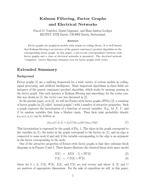
Kalman Filtering,Factor Graphsand Electrical NetworksPascal O.Vontobel,Daniel Lippuner,and Hans-Andrea LoeligerISI-ITET,ETH Zurich,CH-8092Zurich,Switzerland.AbstractFactor graphs are graphical models with origins in coding theory.It is well known that Kalmanﬁltering is an instance of the generic sum(mary)-product algorithm on thecorresponding factor graph.In this paper,a one-to-one correspondence between suchfactor graphs and a class of electrical networks is presented.The electrical network“computes”correct Bayesian estimates even for factor graphs with cycles. Extended SummaryBackgroundFactor graphs[1]are a unifying framework for a wide variety of system models in coding, signal processing,and artiﬁcial intelligence.Many important algorithms in theseﬁelds are instances of the generic sum(mary)-product algorithm,which works by message passing in the factor graph.One such instance is Kalmanﬁltering and smoothing;for the scalar case, this was shown in[1],the vector case was discussed in[2].In the present paper,as in[2],we will use Forney-style factor graphs(FFGs)[3],a variation of factor graphs(in[3]called“normal graphs”)with a number of attractive properties.Such a graph expresses the factorization of a function of several variables. E.g.,let X,Y,and Z be random variables that form a Markov chain.Then their joint probability density p XY Z(x,y,z)can be written asp XY Z(x,y,z)=p X(x)p Y|X(y|x)p Z|Y(z|y).(1)This factorization is expressed by the graph of Fig.1.The edges in the graph correspond to the variables in(1),the nodes in the graph correspond to the factors in(1),and an edge is connected to some node if and only if the variable corresponding to the edge is an argument in the factor corresponding to the node.One of the attractive properties of Forney-style factor graphs is that they subsume block diagrams as in Figures2and3.Theseﬁgures illustrate the classical linear state space modelX[k]=AX[k−1]+BU[k](2)Y[k]=CX[k]+W[k](3)where for k∈Z,U[k],W[k],X[k],and Y[k]are real vectors and where A,B,and C are matrices of appropriate dimensions.For the sake of exposition we will,in this paper,focus on the case where all these variables and matrices are scalars.The nodes in Figures 2and3are then deﬁned to represent factors as shown in Table1(left column).In Kalman ﬁltering,both U[.]and W[.]are usually assumed to be white Gaussian(“noise”)processes; the corresponding nodes in theseﬁgures are then of the type shown in the top row of Table1. The overall function(the factorization of)which is expressed by Figures2and3is the joint probability density of all involved variables.If the variables Y[k]are observed,say Y[k]=y k,the corresponding branches are“ter-minated”by nodes corresponding to factorsδ(y[k]−y k)(the dashed boxes in Fig.2);such factors may be viewed as degenerate cases of Gaussian distributions(top row of Table1) with variance zero.The graph then represents(the factorization of)the joint a posteriori density of all involved variables.As described in[1]and[2],Kalmanﬁltering may be viewed as passing messages along the edges of these graphs;in general,the messages consist of mean vectors and covariance matrices(or inverses of covariance matrices)and are computed according to the rules of the generic sum-product algorithm.In its most narrow sense,Kalmanﬁltering is only the forward sum-product recursion through the graph of Fig.2and yields the a posteriori probability distribution of the state X[k]given the observation sequence Y[.]up to time k.By computing also the backwards messages,the a posteriori probability of all quantities given the whole observation sequence Y[.]may be obtained.More generally,Kalmanﬁltering amounts to the sum-product algorithm on any FFG(or part of an FFG)that consists of(the vector/matrix versions of)the linear building blocks listed in Table1(left column).As pointed out in[2],Kalmanﬁltering in this sense is equivalent to a general least-squares algorithm.New ResultsInterestingly,the results of Kalmanﬁltering(in its widest sense as deﬁned above)can also be obtained by translating the state space model into an electrical network according to the rules of Table1.These networks consist of resistors,voltage sources,and transformers. (The latter are deﬁned by the equations U2=aU1and I2=I1/a,where U i and I i are the voltage accross,and the current into,terminal pair i,i=1,2.)As shown in Table1,each edge/variable of the factor graph corresponds to a pair of nodes in the electrical network.Theorem.The voltages between such node pairs are the Bayesian estimates(i.e.,the means of the a posteriori marginal distributions)of the corresponding random variables.The equivalence of(traditional)Kalmanﬁltering with an electrical network as in Table1 was recognized already by Carter[4].However,the above theorem holds also if the factor graph has cycles,which goes beyond[4](and appears to be related to the convergence results of[6]and[7]).In the electrical network,message passing according to the sum-product algorithm(and thus classical Kalmanﬁltering)can be interpreted as follows.Each message represents aGaussian distribution as in the top row of Table1,and can thus be represented by a voltage source(corresponding to the mean)in series with a resistor(corresponding to the variance). As illustrated in Table2,the computation of messages out of the other node types in Table1 then amounts to connecting the incoming messages/circuits to the node circuit and reducing the resulting circuit to its Th´e venin equivalent circuit(i.e.,a voltage source in series with a resistor).We conclude with the following remarks:•The correspondence given in Table1can be extended to the vector case.•There is a dual version of the correspondence of Table1where the voltages and the currents are interchanged,as are series and parallel connections of subcircuits.•The representation of Kalmanﬁltering(and smoothing)as an electrical network al-lows an easy transition from discrete-time Kalmanﬁltering to continuous-time Kalman ﬁltering.•A generalization beyond Kalmanﬁltering/least squares was recently discovered by theﬁrst author[8]:if p(x,y,...)is any joint probability density function such that −log p(x,y,...)is convex,then a factor graph of p can be translated into an electrical network thatﬁnds the global maximum of p.The network consists of voltage sources (or current sources)and nonlinear resistors.Circuit simpliﬁcations similar to those in Table2correspond to the message passing rules of the max-product version(rather than the sum-product version)of generic sum(mary)-product algorithm.Moreover,if the voltages are solutions to the primal maximization problem,then the currents are the solutions to the dual problem.AcknowledgementThe authors thank S.Mitter for pointing out the book by Dennis[5],which inspired this work.p X Xp Y |X Y p Z |Y ZFigure 1:Forney-style factor graph (FFG)of a Markov chain....-X [k −1]?U [k ]?Z [k ]?Y [k ]-X [k ]?U [k +1]?Z [k +1]?Y [k +1]-X [k +1]...Figure 2:State space model.-X [k −1]A -?U [k ]B?+-=?C ?Z [k ]-X [k ]-W [k ]?Z [k ]+?Y [k ]Figure 3:Details of linear state space model.γe−(x −m )22σ2Xm ?m σ2?X 1δ(x −y )δ(x −z )=XZ Y r r?X ?Z -Y 2δ(x +y −z )+-X -Z 6Y?X ?Z -Y 3δ(y −ax )a-X -Y ¤¥¤¥¤¥§¦§¦§¦1:a ?X?Y Table 1:Correspondence between the nodes in the factor graph (left)and the components of the electrical network (right).All variables are scalars.1=X-Z -Y 6m Z =m X /σ2X +m Y /σ2Y 1/σ2X +1/σ2Y σ2Z =11/σ2X +1/σ2Y j σ2X m X j σ2Y m Y r r ⇒j σ2Z m Z2+-X --Z -6Y 6m Z =m X +m Y σ2Z =σ2X +σ2Y j σ2X m X j m Y σ2Y ⇒j σ2Z m Z3a -X --Y -m Y =am Xσ2Y =a 2σ2X j σ2X m X ¤¥¤¥¤¥§¦§¦§¦1:a⇒j σ2Y m YTable 2:Computation of messages (left and middle)with circuit interpretation (right).References[1] F.R.Kschischang,B.J.Frey,and H.-A.Loeliger,“Factor graphs and the sum-product algo-rithm,”IEEE rm.Theory,vol.IT–47,no.2,pp.498–519,2001.[2]H.-A.Loeliger,“Least squares and Kalmanﬁltering on Forney graphs,”to appear in Codes,Graphs,and Systems,festschrift in honour of G.D.Forney,Kluwer,2001.[3]G.D.Forney,Jr.,“Codes on graphs:normal realizations,”IEEE rm.Theory,vol.IT-47,pp.520–548,Feb.2001.[4] D.W.Carter,“A circuit theory of the Kalmanﬁlter,”in Proc.32nd Conf.on Decision andControl(San Antonio,TX,USA),pp.1224–1226,Dec.1993.[5]J.B.Dennis,Mathematical Programming and Electrical Networks.MIT Press,Cambridge,Mass.,1959.[6]Y.Weiss and W.T.Freeman,“On the optimality of solutions of the max-product belief-propagation algorithm in arbitrary graphs,”IEEE rm.Theory,vol.47,pp.736–744, Feb.2001.[7]P.Rusmevichientong and B.Van Roy,“An analysis of belief propagation on the turbo decodinggraph with Gaussian densities,”IEEE rm.Theory,vol.47,pp.745–765,Feb.2001.[8]P.O.Vontobel,Kalman Filters,Factor Graphs,and Electrical Networks.Internal reportINT/200202,ISI-ITET,ETH Zurich,April2002.。

Multilayer networks

1. Introduction Network theory is an important tool for describing and analysing complex systems throughout the social, biological, physical, information and engineering sciences [1–3]. Originally, almost all studies of networks employed an abstraction in which systems are represented as ordinary graphs [4]: the ‘nodes’ (or ‘vertices’) of the graphs represent some entity or agent, and a tie between a pair of nodes is represented using a single, static, unweighted ‘edge’ (or ‘link’). Self- and multi-edges were also typically ignored. Although this approach is naive in many respects, it has been extremely successful. For example, it has been used to illustrate that many real networks possess a heavy-tailed degree distribution [5,6], exhibit the small-world property [7,8], contain nodes that play central roles [1,2] and/or have modular structures [9–11]. As research on complex systems has matured, it has become increasingly essential to move beyond simple graphs and investigate more complicated but more realistic frameworks. For example, edges often exhibit heterogeneous features: they can be directed [1,2,12], have different strengths (i.e. ‘weights’) [2,13,14], exist only between nodes that belong to different sets (e.g. bipartite networks) [1,2, 15] or be active only at certain times [16,17]. Most recently, there have been increasingly intense efforts to investigate networks with multiple types of connections (see Section 2.5) and so-called ‘network of networks’1 [19] (see Section 2.4). Such systems were examined decades ago in disciplines like sociology and engineering, but the explosive attempt to develop frameworks to study multilayer complex systems and to generalize a large body of familiar tools from network science is a recent phenomenon.2 In social networks, one can categorize edges based on the nature of the relationships (i.e. ties) or actions that they represent [2,21,22]. Reducing a social system to a network in which actors are connected in a pairwise fashion by only a single type of relationship is often an extremely crude approximation of reality. As a result, sociologists recognized decades ago that it is crucial to study social systems by constructing multiple social networks using different types of ties among the same set of individuals [2,23].3 For example, consider the sociograms4 that were drawn in the 1930s to represent social networks in a bank-wiring room [26]. These sociograms depicted relations between 14 individuals via 6 different types of social interactions (see Fig. 6(b)). In the sociology literature, networks in which each edge is categorized by its type are called ‘multiplex networks’ [27,28] or ‘multirelational networks’ [2]. (Such networks are also said to possess ‘multi-stranded’ relationships [29].) Social networks also often include several types of nodes (e.g. males and females) or hierarchical structures (e.g. individuals are part of organizations), which have been studied using ‘multilevel networks’ (see Section 2.8). The notion of a ‘network of networks’ also dates at least as far back as 1973 [30]. The tools

折线图英语作文

折线图英语作文Title: Exploring the Significance of Line Graphs。

Introduction:Line graphs are an indispensable tool in data representation, widely used across various fields such as economics, science, and social sciences. Their simplicity and effectiveness in illustrating trends and patterns make them a preferred choice for conveying information. In this essay, we delve into the importance and utility of line graphs.Importance of Line Graphs:Line graphs serve multiple purposes, primarily to visualize and analyze data trends over time or other continuous variables. They offer a clear depiction of how one variable changes in relation to another, aiding in the identification of patterns, correlations, and anomalies.1. Trend Analysis:One of the fundamental applications of line graphs is to analyze trends. By plotting data points over time, line graphs provide insights into the direction and magnitude of change in variables. For instance, in economic analysis, line graphs are used to track GDP growth, unemployment rates, or stock market performance over different periods.2. Comparisons:Line graphs facilitate easy comparison betweendifferent datasets. Multiple lines on the same graph enable viewers to contrast trends and observe any disparities or similarities. This is particularly useful in fields like marketing, where companies can compare sales figures of various products or services over time.3. Forecasting:Line graphs can also aid in forecasting future trendsbased on past data. By extrapolating the existing trend lines, analysts can make informed predictions about future outcomes. This forecasting capability is valuable in financial planning, resource allocation, and risk management.4. Identification of Patterns:Line graphs help in identifying underlying patterns within datasets. Whether it's seasonal fluctuations, cyclical trends, or long-term growth trajectories, line graphs provide a visual framework for pattern recognition. This assists researchers and decision-makers in understanding the underlying dynamics driving the data.5. Communication of Findings:In addition to their analytical functions, line graphs are powerful communication tools. They simplify complex data into visually appealing representations that are easy to comprehend. Whether presenting to stakeholders, policymakers, or the general public, line graphs facilitateeffective communication of findings and insights.Example Applications:To illustrate the versatility of line graphs, consider the following examples:1. Climate Change Analysis:Line graphs are commonly used to visualize temperature trends over decades. By plotting annual average temperatures, scientists can demonstrate the long-term impact of climate change, highlighting the steady rise in global temperatures.2. Stock Market Performance:Investors rely on line graphs to track the performance of stocks, indices, and commodities. A line graph depicting the movement of a stock price over time helps investors identify patterns, assess volatility, and make informed trading decisions.3. Disease Outbreak Monitoring:Health organizations utilize line graphs to monitor the spread of diseases such as COVID-19. By plotting daily or weekly case counts, epidemiologists can track the progression of outbreaks, assess the effectiveness of interventions, and forecast future infection rates.Conclusion:In conclusion, line graphs play a crucial role in data analysis, interpretation, and communication. Their ability to represent trends, compare datasets, forecast future outcomes, identify patterns, and communicate findings makes them an indispensable tool across various domains. As we continue to navigate an increasingly data-driven world, the importance of line graphs in understanding complex phenomena cannot be overstated.。

软件工程_东北大学中国大学mooc课后章节答案期末考试题库2023年

软件工程_东北大学中国大学mooc课后章节答案期末考试题库2023年1._______ is a discipline whose aim is the production of fault-free software,delivered on time and within budget, that satisfies the client's needs._______是一个学科，其目标是生产出满足客户的需求的、未超出预算的、按时交付的、没有错误的软件。

答案:2.The relationship between whole-class and part-classes is called ______.整体和部分类之间的关系被称为______。

答案:aggregation3.The relationship between super-class and subclasses is called ______.超类和子类之间的关系称为______。

答案:inheritance4.The strategy of inheritance is to use inheritance wherever _______.继承的策略是在_______的情况下使用继承。

答案:appropriate5._____is to encapsulate the attributes and operations in an object, and hides theinternal details of an object as possible. _____是为了在一个对象中封装属性和操作，并尽可能隐藏对象的内部细节。

Data encapsulation6.Two modules are ________ coupled if they have write access to global data.如果两个模块对全局数据具有写访问权限，则是________耦合。

《软件需求分析、设计与建模》简答题样题1(含答案)

1．What is object technology? What do you perceive as object technology’s strength? It’s weakness?Object【A set of principles (abstraction, encapsulation, polymorphism) guiding software construction, together with languages, databases, and other tools that support those principles.】面向对象技术是一系列支持软件开发的原则（抽象，封装，多态性），以及支持这些原则的程序设计语言，数据库和其它工具。

【Reflects a single paradigm.Facilitates architectural and code reuse.Reflects real world models more closely.Encourages stability.Is adaptive to change】反映一个特定实例。

有利于构件和代码重用。

更加真实地反映现实世界模型。

具有更好的稳定性。

能适应需求的变化。

2．What is UML? List at least three benefits of developing with UML.【UML is Unified Modeling Language, it is a language for Visualizing, Specifying, Constructing, Documenting the artifacts of a software-intensive system. 】UML是统一建模语言，是一门用于对面向对象开发的产品进行可视化建模，说明，架构和文档编制的标准语言。

International Conference on Principles and Practice of Constraint Programming 1995, pp.88–

International Conference on Principles and Practice of Constraint Programming1995,pp.88–102 Asynchronous Weak-commitment Search for Solving Distributed Constraint SatisfactionProblemsMakoto YokooNTT Communication Science Laboratories2-2Hikaridai,Seika-cho,Soraku-gun,Kyoto619-02,Japane-mail:yokoo@cslab.kecl.ntt.jpAbstract.A distributed constraint satisfaction problem(DistributedCSP)is a CSP in which variables and constraints are distributed amongmultiple automated agents,and various application problems in Dis-tributed Artiﬁcial Intelligence can be formalized as Distributed CSPs.We develop a new algorithm for solving Distributed CSPs called asyn-chronous weak-commitment search,which is inspired by the weak-commit-ment search algorithm for solving CSPs.This algorithm can revise a baddecision without an exhaustive search by changing the priority orderof agents dynamically.Furthermore,agents can act asynchronously andconcurrently based on their local knowledge without any global control,while guaranteeing the completeness of the algorithm.The experimental results on various example problems show that thisalgorithm is by far more eﬃcient than the asynchronous backtrackingalgorithm for solving Distributed CSPs,in which the priority order isstatic.The priority order represents a hierarchy of agent authority,i.e.,the priority of decision making.Therefore,these results imply that aﬂexible agent organization,in which the hierarchical order is changeddynamically,actually performs better than an organization in which thehierarchical order is static and rigid.1IntroductionDistributed Artiﬁcial Intelligence(DAI)is a subﬁeld of AI that is concerned with the interaction,especially the coordination among artiﬁcial automated agents. Since distributed computing environments are spreading very rapidly due to the advances in hardware and networking technologies,there are pressing needs for DAI techniques,thus DAI is becoming a very vital area in AI.In[13],a distributed constraint satisfaction problem(Distributed CSP)is formalized as a CSP in which variables and constraints are distributed among multiple automated agents.It is well known that surprisingly a wide variety of AI problems can be formalized as CSPs.Similarly,various application problems in DAI which are concerned withﬁnding a consistent combination of agent ac-tions(e.g.,distributed resource allocation problems[3],distributed scheduling problems[9],and multi-agent truth maintenance tasks[5])can be formalized as Distributed CSPs.Therefore,we can consider a Distributed CSP as a generalframework for DAI,and distributed algorithms for solving Distributed CSPs as an important infrastructure in DAI.It must be noted that although algorithms for solving Distributed CSPs seem to be similar to parallel/distributed processing methods for solving CSPs[2,14], research motivations are fundamentally diﬀerent.The primary concern in par-allel/distributed processing is the eﬃciency,and we can choose any type of par-allel/distributed computer architecture for solving the given problem eﬃciently. In contrast,in a Distributed CSP,there already exists a situation where knowl-edge about the problem(i.e.,variables and constraints)is distributed among automated agents.Therefore,the main research issue is how to reach a solution from this given situation.If all knowledge about the problem can be gathered into one agent,this agent can solve the problem alone using normal centralized constraint satisfaction algorithms.However,collecting all information about a problem requires certain communication costs,which could be prohibitively high. Furthermore,in some application problems,gathering all information to one agent is not desirable or impossible for security/privacy reasons.In such cases, multiple agents have to solve the problem without centralizing all information. The author has developed a basic algorithm for solving Distributed CSPs called asynchronous backtracking[13].In this algorithm,agents act asynchronously and concurrently based on their local knowledge without any global control.In this paper,we develop a new algorithm called asynchronous weak-commit-ment search,which is inspired by the weak-commitment search algorithm for solving CSPs[12].The main characteristic of this algorithm is as follows.–Agents can revise a bad decision without an exhaustive search by changing the priority order of agents dynamically.In the asynchronous backtracking algorithm,the priority order of agents is de-termined,and an agent tries toﬁnd a value satisfying the constraints with the variables of higher priority agents.When an agent sets a variable value,the agent commits to the selected value strongly,i.e.,the selected value will not be changed unless an exhaustive search is performed by lower priority agents.There-fore,in large-scale problems,a single mistake of value selection becomes fatal since doing such an exhaustive search is virtually impossible.This drawback is common to all backtracking algorithms.On the other hand,in the asynchronous weak-commitment search,when an agent can notﬁnd a value consistent with the higher priority agents,the priority order is changed so that the agent has the highest priority.As a result,when an agent makes a mistake in value se-lection,the priority of another agent becomes higher;thus the agent that made the mistake will not commit to the bad decision,and the selected value will be changed.We will show that the asynchronous weak-commitment search algorithm can solve problems such as the distributed1000-queens problem,the distributed graph-coloring problem,and the network resource allocation problem[8]that the asynchronous backtracking algorithm fails to solve within a reasonable amount of time.We can assume that the priority order represents a hierarchy of agentauthority,i.e.,the priority order of decision making.Therefore,these results im-ply that aﬂexible agent organization,in which the hierarchical order is changed dynamically,actually performs better than an organization in which the hierar-chical order is static and rigid.In the following,we brieﬂy describe the deﬁnition of a Distributed CSP and the asynchronous backtracking algorithm(Section2).Then,we show the basic ideas and details of the asynchronous weak-commitment search algorithm(Sec-tion3),and empirical results which show the eﬃciency of the algorithm(Section 4).Finally,we examine the complexity of the algorithm(Section5).2Distributed Constraint Satisfaction Problem and Asynchronous Backtracking2.1FormalizationA CSP consists of n variables x1,x2,...,x n,whose values are taken fromﬁ-nite,discrete domains D1,D2,...,D n respectively,and a set of constraints on their values.A constraint is deﬁned by a predicate.That is,the constraint p k(x k1,...,x kj)is a predicate which is deﬁned on the Cartesian product D k1×...×D kj.This predicate is true iﬀthe value assignment of these variables sat-isﬁes this constraint.Solving a CSP is equivalent toﬁnding an assignment of values to all variables such that all constraints are satisﬁed.A Distributed CSP is a CSP in which variables and constraints are distributed among automated agents.We assume the following communication model.–Agents communicate by sending messages.An agent can send messages to other agents iﬀthe agent knows the addresses of the agents1.–The delay in delivering a message isﬁnite,though random.For the trans-mission between any pair of agents,messages are received in the order in which they were sent.Each agent has some variables and tries to determine their values.However, there exist inter-agent constraints,and the value assignment must satisfy these inter-agent constraints.Formally,there exist m agents1,2,...,m.Each variable x j belongs to one agent i(this relation is represented as belongs(x j,i)).Con-straints are also distributed among agents.The fact that an agent k knows a constraint predicate p l is represented as known(p l,k).We say that a Distributed CSP is solved iﬀthe following conditions are satisﬁed.1This model does not necessarily mean that the physical communication network must be fully connected(i.e.,a complete graph).Unlike most parallel/distributed algorithm studies,in which the topology of the physical communication network plays an important role,we assume the existence of a reliable underlying commu-nication structure among agents and do not care about the implementation of the physical communication network.This is because our primary concern is the coop-eration of intelligent agents,rather than solving CSPs by certain multi-processor architectures.–∀i,∀x j where belongs(x j,i),the value of x j is assigned to d j,and∀k,∀p l where known(p l,k),p l is true under the assignment x j=d j.2.2Asynchronous BacktrackingA basic algorithm for solving Distributed CSPs called asynchronous backtrack-ing is developed in[13].In this algorithm,agents act asynchronously and con-currently,in contrast to traditional sequential backtracking techniques,while guaranteeing the completeness of the algorithm.Without loss of generality,we make the following assumptions while describ-ing our algorithms for simplicity.Relaxing these assumptions to general cases is relatively straightforward2.–Each agent has exactly one variable.–All constraints are binary.–There exists a constraint between any pair of agents.–Each agent knows all constraint predicates relevant to its variable.In the following,we use the same identiﬁer x i to represent an agent and its variable.We assume that each agent(and its variable)has a unique identiﬁer.In the asynchronous backtracking algorithm,each agent concurrently assigns a value to its variable,and sends the value to other agents.After that,agents wait for and respond to incoming messages.There are two kinds of messages: ok?messages to communicate the current value,and nogood messages to com-municate information about constraint violations.The procedures executed at agent x i by receiving an ok?message and a nogood message are described in Fig.1.An overview of these procedures is given as follows.–After receiving an ok?message,an agent records the values of other agents in its agent view.The agent view represents the state of the world recognized by this agent(Fig.1(i)).–The priority order of variables/agents is determined by the alphabetical or-der of the identiﬁers,i.e.,preceding variables/agents in the alphabetical or-der have higher priority.If the current value satisﬁes the constraints with higher priority agents in the agent view,we say that the current value is consistent with the agent view3.If the current value is not consistent with the agent view,the agent selects a new value which is consistent with the agent view(Fig.1(ii)).2In[11],an algorithm in which each agent has multiple variables is described.If there exists no explicit constraint between two agents,there is a chance that an implicit constraint exists between them.In such a case,a new relation between these agents must be generated dynamically.The procedure for adding a new relation is described in[13].The idea of making originally implicit constraints explicit can be found in the consistency algorithms for CSPs.For example,the adaptive consistency procedure[4]adds links to a constraint network while transforming the constraint network toa backtrack-free constraint network.3More precisely,the agent must satisfy not only initially given constraint predicates, but also the new constraints communicated by nogood messages.–If the agent can notﬁnd a value consistent with the agent view,the agent sends nogood messages to higher priority agents(Fig.1(iii)).A nogood mes-sage contains a set of variable values that can not be a part of anyﬁnal solution.By using this algorithm,if a solution exists,agents will reach a stable state where all constraints are satisﬁed.If there exists no solution,an empty nogood will be found and the algorithm will terminate4.when received(ok?,(x j,d j))do—(i)add(x j,d j)to agent view;check agent view;end do;when received(nogood,x j,nogood)doadd nogood to nogood list;check agent view;end do;procedure check agent viewwhen agent view and current value are not consistent do—(ii)if no value in D i is consistent with agent view then backtrack;—(iii)else select d∈D i where agent view and d are consistent;current value←d;send(ok?,(x i,d))to other agents;end if;end do;procedure backtracknogoods←{V|V=inconsistent subset of agent view};when an empty set is an element of nogoods dobroadcast to other agents that there is no solution,terminate this algorithm;end do;for each V∈nogoods do;select(x j,d j)where x j has the lowest priority in V;send(nogood,x i,V)to x j;end do;Fig.1.Procedures for receiving messages(asynchronous backtracking)4A set of variable values that is a superset of a nogood can not be aﬁnal solution.If an empty set becomes a nogood,it means that there is no solution,since any set is a superset of an empty set.3Asynchronous Weak-commitment SearchIn this section,we brieﬂy describe the weak-commitment search algorithm for solving CSPs[12],and describe how the asynchronous backtracking algorithm can be modiﬁed into the asynchronous weak-commitment search algorithm. 3.1Weak-commitment Search AlgorithmIn the weak-commitment search algorithm(Fig.2),all variables have tentative initial values.We can execute this algorithm by calling weak-commitment ({(x1,d1),(x2,d2),...,(x n,d n)},{}),where d i is the tentative initial value of x i.In this algorithm,a consistent partial solution is constructed for a subset ofvariables,and this partial solution is extended by adding variables one by one un-til a complete solution is found.When a variable is added to the partial solution, its tentative initial value is revised so that the new value satisﬁes all constraints between the partial solution,and satisﬁes as many constraints between variables that are not included in the partial solution as possible.This value ordering heuristic is called the min-conﬂict heuristic[6].The essential diﬀerence between this algorithm and the min-conﬂict backtracking[6]is the underlined part in Fig.2.When there exists no value for one variable that satisﬁes all constraints between the partial solution,this algorithm abandons the whole partial solution, and starts constructing a new partial solution from scratch,using the current value assignment as new tentative initial values.This algorithm records the abandoned partial solutions as new constraints, and avoids creating the same partial solution that has been created and aban-doned before.Therefore,the completeness of the algorithm(alwaysﬁnds a so-lution if one exists,and terminates if no solution exists)is guaranteed.The experimental results on various example problems in[12]show that this algo-rithm is3to10times more eﬃcient than the min-conﬂict backtracking[6]or the breakout algorithm[7].3.2Basic IdeasThe main characteristics of the weak-commitment search algorithm are as fol-lows.1.The algorithm uses the min-conﬂict heuristic as a value ordering heuristic.2.It abandons the partial solution and restarts the search process if there existsno consistent value with the partial solution.Introducing theﬁrst characteristic into the asynchronous backtracking algo-rithm is relatively straightforward.When selecting a variable value,if there exist multiple values consistent with the agent view(those that satisfy all constraints with variables of higher priority agents),the agent prefers the value that mini-mizes the number of constraint violations with variables of lower priority agents.In contrast,introducing the second characteristic into the asynchronous back-tracking is not straightforward,since agents act concurrently and asynchronously,procedure weak-commitment(left,partial-solution)when all variables in left satisfy all constraints doterminate the algorithm,current value assignment is a solution;end do (x i,d)←a variable and value pair in left that does not satisfy some constraint;values←the list of x i’s values that are consistent with partial-solution;if values is an empty list;if partial-solution is an empty listthen terminate the algorithm since there exists no solution;else record partial-solution as a new constraint(nogood);remove each element of partial-solution and add to left;call weak-commitment(left,partial-solution);end if;else value←the value within values that minimizesthe number of constraint violations with left;remove(x i,d)from left;add(x i,value)to partial-solution;call weak-commitment(left,partial-solution);end if;Fig.2.Weak-commitment search algorithmand no agent has exact information about the partial solution.Furthermore, multiple agents may try to restart the search process simultaneously.In the following,we show that the agents can commit to their decisions weakly by changing the priority order dynamically.We deﬁne the way of establishing the priority order by introducing priority values,and change the priority values by the following rules.–For each variable/agent,a non-negative integer value representing the pri-ority order of the variable/agent is deﬁned.We call this value the priority value.–The order is deﬁned such that any variable/agent with a larger priority value has higher priority.–If the priority values of multiple agents are the same,the order is determined by the alphabetical order of the identiﬁers.–For each variable/agent,the initial priority value is0.–If there exists no consistent value for x l,the priority value of x l is changed to k+1,where k is the largest priority value of other agents.Furthermore,in the asynchronous backtracking algorithm,agents try to avoid situations previously found to be nogoods.However,due to the delay of mes-sages,an agent view of an agent can occasionally be a superset of a previously found nogood.In order to avoid reacting to unstable situations,and perform-ing unnecessary changes of priority values,each agent performs the following procedure.–Each agent records the nogoods that it has sent.When the agent view is a superset of a nogood that it has already sent,the agent will not change the priority value and waits for the next message.3.3Details of AlgorithmIn the asynchronous weak-commitment search,each agent concurrently assigns avalue to its variable,and sends the value to other agents.After that,agents wait for and respond to incoming messages5.In Fig.3,the procedures executed atagent x i by receiving an ok?message and a nogood message are described6.Thediﬀerences between these procedures and the procedures for the asynchronous backtracking algorithm are as follows.–The priority value,as well as the current value,is communicated throughthe ok?message(Fig.3(i)).–The priority order is determined by the communicated priority values.Ifthe current value is not consistent with the agent view,i.e.,some constraintwith variables of higher priority agents is not satisﬁed,the agent changes its value so that the value is consistent with the agent view,and also thevalue minimizes the number of constraint violations with variables of lower priority agents(Fig.3(ii)).–When x i can notﬁnd a consistent value with its agent view,x i sends nogoodmessages to other agents,and increments its priority value.If x i has already sent an identical nogood,x i will not change the priority value and will waitfor the next message(Fig.3(iii)).3.4Example of Algorithm ExecutionWe illustrate the execution of the algorithm using a distributed version of the well-known n-queens problem(where n=4).There exist four agents,each ofwhich corresponds to a queen of each row.The goal of the agents is toﬁnd positions on a4×4chess board so that they do not threaten one another.The initial values are shown in Fig.4(a).Agents communicate these valuesto one another.The values within parentheses represent the priority values.The initial priority values are0.Since the priority values are equal,the priority orderis determined by the alphabetical order of identiﬁers.Therefore,only the value ofx4is not consistent with its agent view,i.e.,only x4is violating constraints with higher priority agents.Since there is no consistent value,agent x4sends nogoodmessages and increments its priority value.In this case,the value minimizing the number of constraint violations is3,since it conﬂicts only with x3.Therefore, x4selects3and sends ok?messages to other agents(Fig.4(b)).Then,x3tries to change its value.Since there is no consistent value,agent x3sends nogood messages,and increments its priority value.In this case,the value that minimizes 5Although the following algorithm is described in a way that an agent reacts to messages sequentially,an agent can handle multiple messages concurrently,i.e.,the agentﬁrst revises agent view and nogood list according to the messages,and performs check agent view only once.6It must be mentioned that the way to determine that agents as a whole have reached a stable state is not contained in this algorithm.To detect the stable state,agents must use distributed termination detection algorithms such as[1].when received(ok?,(x j,d j,priority))do—(i)add(x j,d j,priority)to agent view;check agent view;end do;when received(nogood,x j,nogood)doadd nogood to nogood list;check agent view;end do;procedure check agent viewwhen agent view and current value are not consistent doif no value in D i is consistent with agent view then backtrack;else select d∈D i where agent view and d are consistentand d minimizes the number of constraint violations;—(ii)current value←d;send(ok?,(x i,d,current priority))to other agents;end if;end do; procedure backtrack—(iii)nogoods←{V|V=inconsistent subset of agent view};when an empty set is an element of nogoods dobroadcast to other agents that there is no solution,terminate this algorithm;end do;when no element of nogoods is included in nogood sent dofor each V∈nogoods do;add V to nogood sentfor each(x j,d j)in V do;send(nogood,x i,V)to x j;end do;end do;p max←max(x j,d j,p j)∈agent view(p j);current priority←1+p max;select d∈D i where d minimizes the number of constraint violations;current value←d;send(ok?,(x i,d,current priority))to other agents;end do;Fig.3.Procedures for receiving messages(asynchronous weak-commitment search)the number of constraint violations is1or2.In this example,x3selects1and sends ok?messages to other agents(Fig.4(c)).After that,x1changes its value to2,and a solution is obtained(Fig.4(d)).In the distributed4-queens problem,there exists no solution when x1’s value is1.We can see that a bad decision can be revised without an exhaustive search in the asynchronous weak-commitment search.x 1x 2x 3x 4(a)(b)(c)(d)(0)(0)(0)(1)(0)(0)(2)(1)(0)(0)(2)(1)Fig.4.Example of algorithm execution3.5Algorithm CompletenessThe priority values are changed if and only if a new nogood is found 7.Since the number of possible nogoods is ﬁnite,the priority values can not be changed inﬁnitely.Therefore,after a certain time point,the priority values will be stable.Then,we show that the situations described below will not occur when the priority values are stable.(i)There exist agents that do not satisfy some constraints,and all agents are waiting for incoming messages.(ii)Messages are repeatedly sent/received,and the algorithm will not reach a stable state (inﬁnite processing loop).If situation (i)occurs,there exist at least two agents that do not satisfy the constraint between them.Let us assume that the agent ranking k-th in the priority order does not satisfy the constraint between the agent ranking j-th (where j <k ),and all agents ranking higher than k-th satisfy all constraints within them.The only case that the k-th agent waits for incoming messages even though the agent does not satisfy the constraint between the j-th agent is that the k-th agent has sent nogood messages to higher priority agents.This fact contradicts the assumption that higher priority agents satisfy constraints within them.Therefore,situation (i)will not occur.Also,if the priority values are stable,the asynchronous weak-commitment search algorithm is basically identical to the asynchronous backtracking algo-rithm.Since the asynchronous backtracking is guaranteed not to fall into an inﬁnite processing loop [13],situation (ii)will not occur.From the fact that situation (i)or (ii)will not occur,we can guarantee that the asynchronous weak-commitment search algorithm will always ﬁnd a solution,or ﬁnd the fact that there exists no solution.4EvaluationsIn this section,we evaluate the eﬃciency of algorithms by discrete event sim-ulation,where each agent maintains its own simulated clock.An agent’s time 7To be exact,diﬀerent agents may ﬁnd an identical nogood simultaneously.is incremented by one simulated time unit whenever it performs one cycle of computation.One cycle consists of reading all incoming messages,performing local computation,and sending messages.We assume that a message issued at time t is available to the recipient at time t+1.We analyze performance in terms of the amount of cycles required to solve the problem.Given this model, we compare the following three kinds of algorithms:(a)asynchronous backtrack-ing,in which a variable value is selected randomly from consistent values,and the priority order is determined by alphabetical order,(b)min-conﬂict only,in which the min-conﬂict heuristic is introduced into the asynchronous backtrack-ing,but the priority order is statically determined by alphabetical order,and(c) asynchronous weak-commitment search8.Weﬁrst applied these three algorithms to the distributed n-queens problem described in the previous section,varying n from10to1000.The results are summarized in Table1.For each n,we generated100problems,each of which had diﬀerent randomly generated initial values,and averaged the results for these problems.For each problem,in order to conduct the experiments in a reasonable amount of time,we set the bound for the number of cycles to1000, and terminated the algorithm if this limit was exceeded;we counted the result as1000.The ratio of problems completed successfully to the total number of problems is also described in Table1.Table1.Required cycles for distributed n-queens problemasynchronous min-conﬂict only asynchronousbacktracking weak-commitmentn ratio cycles ratio cycles ratio cycles10100%105.4100%102.6100%41.55050%662.756%623.0100%59.110014%931.430%851.3100%50.810000%—16%891.8100%29.6 The second example problem is the distributed graph-coloring problem.The distributed graph-coloring problem is a graph-coloring problem,in which each node corresponds to an agent.The graph-coloring problem involves painting nodes in a graph by k diﬀerent colors so that any two nodes connected by an arc do not have the same color.We randomly generate a problem with n nodes/agents and m arcs by the method described in[6],so that the graph is connected and the problem has a solution.We evaluate the problem n=60,90,8The amounts of local computation performed in each cycle for(b)and(c)are equiv-alent.The amounts of local computation for(a)can be smaller since it does not use the min-conﬂict heuristic,but for the lowest priority agent,the amounts of local computation of these algorithms are equivalent.。

Neo4j教程：基础到高级概念说明书

About the T utorialNeo4j is one of the popular Graph Databases and Cypher Query Language (CQL). Neo4j is written in Java Language. This tutorial explains the basics of Neo4j, Java with Neo4j, and Spring DATA with Neo4j.The tutorial is divided into sections such as Neo4j Introduction, Neo4j CQL, Neo4j CQL Functions, Neo4j Admin, etc. Each of these sections contain related topics with simple and useful examples.AudienceThis tutorial has been prepared for beginners to help them understand the basic to advanced concepts of Neo4j. It will give you enough understanding on Neo4j from where you can take yourself to a higher level of expertise.PrerequisitesBefore proceeding with this tutorial, you should have basic knowledge of Database, Graph Theory, Java, and Spring Framework.Copyright & Disclaimer© Copyright 2018 by Tutorials Point (I) Pvt. Ltd.All the content and graphics published in this e-book are the property of Tutorials Point (I) Pvt. Ltd. The user of this e-book is prohibited to reuse, retain, copy, distribute or republish any contents or a part of contents of this e-book in any manner without written consent of the publisher.We strive to update the contents of our website and tutorials as timely and as precisely as possible, however, the contents may contain inaccuracies or errors. Tutorials Point (I) Pvt. Ltd. provides no guarantee regarding the accuracy, timeliness or completeness of our website or its contents including this tutorial. If you discover any errors on our website or in this tutorial, please notify us at **************************T able of ContentsAbout the Tutorial (i)Audience (i)Prerequisites (i)Copyright & Disclaimer (i)Table of Contents (ii)1.Neo4j ─ Overview (1)What is a Graph Database? (1)Advantages of Neo4j (2)Features of Neo4j (2)2.Neo4j ─ Data Model (4)3.Neo4j ─ Environment Setup (6)Neo4j Database Server Setup with Windows exe File (6)Starting the Server (9)Working with Neo4j (11)4.Neo4j ─ Building Blocks (12)Node (12)Properties (12)Relationships (13)Labels (14)Neo4j Data Browser (14)NEO4J ─ CQL (17)5.Neo4j CQL ─ I ntroduction (18)Neo4j CQL Clauses (18)Neo4j CQL Functions (20)Neo4j CQL Data Types (21)CQL Operators (21)Boolean Operators in Neo4j CQL (22)Comparison Operators in Neo4j CQL (22)6.Neo4j CQL ─ Creating Nodes (24)Creating a Single node (24)Creating Multiple Nodes (27)Creating a Node with a Label (30)Creating a Node with Multiple Labels (33)Create Node with Properties (36)Returning the Created Node (39)7.Neo4j CQL ─ Creating a Relationship (42)Creating Relationships (42)Creating a Relationship Between the Existing Nodes (44)Creating a Relationship with Label and Properties (47)Creating a Complete Path (49)N EO4J CQL ─ WRITE CLA USES (51)8.Neo4j ─ Merge Command (52)Merging a Node with a Label (52)Merging a Node with Properties (56)OnCreate and OnMatch (58)Merge a Relationship (61)9.Neo4j ─ Set Clause (63)Setting a Property (63)Removing a Property (65)Setting Multiple Properties (67)Setting a Label on a Node (69)Setting Multiple Labels on a Node (71)10.Neo4j ─ Delete Clause (74)Deleting All Nodes and Relationships (74)Deleting a Particular Node (75)11.Neo4j ─ Remove Clause (77)Removing a Property (77)Removing a Label From a Node (79)Removing Multiple Labels (81)12.Neo4j ─ Foreach Clause (84)NEO4J CQL ─ READ CLA USES (87)13.Neo4j ─ Match Clause (88)Get All Nodes Using Match (88)Getting All Nodes Under a Specific Label (90)Match by Relationship (92)Delete All Nodes (94)14.Neo4j ─ Optional Match Clause (96)15.Neo4j ─ Where Clause (98)WHERE Clause with Multiple Conditions (101)Using Relationship with Where Clause (103)16.Neo4j ─ Count Function (106)Count (106)Group Count (108)N EO4J CQL ─ GENERAL C LAUSES (111)17.Neo4j ─ Return Clause (112)Returning Nodes (112)Returning Multiple Nodes (114)Returning Relationships (116)Returning Properties (118)Returning All Elements (120)Returning a Variable With a Column Alias (122)18.Neo4j ─ Order By Clause (124)Ordering Nodes by Multiple Properties (126)Ordering Nodes by Descending Order (128)19.Neo4j ─ Limit Clause (131)Limit with expression (133)20.Neo4j ─ Skip Clause (136)Skip Using Expression (138)21.Neo4j ─ With Clause (140)22.Neo4j ─ Unwind Clause (142)NE O4J CQL ─ FUNCTIONS (144)23.Neo4J CQL ─ String Functions (145)String Functions List (145)Upper (145)Lower (147)Substring (149)24.Neo4j ─ Aggreg ation Function (152)AGGREGATION Functions List (152)COUNT (152)MAX (155)MIN (157)AVG (159)SUM (161)N EO4J CQL ─ ADMIN (163)25.Neo4j ─ Backup & Restore (164)Neo4j Database Backup (164)Neo4j Database Restore (171)26.Neo4j ─ Index (174)Creating an Index (174)Deleting an Index (176)27.Neo4j ─ Create Unique Constraint (179)Create UNIQUE Constraint (179)28.Neo4j ─ Drop Unique (182)Neo4j5Neo4j is the world's leading open source Graph Database which is developed using Java technology. It is highly scalable and schema free (NoSQL).What is a Graph Database?A graph is a pictorial representation of a set of objects where some pairs of objects are connected by links . It is composed of two elements - nodes (vertices) and relationships (edges).Graph database is a database used to model the data in the form of graph. In here, the nodes of a graph depict the entities while the relationships depict the association of these nodes. Popular Graph DatabasesNeo4j is a popular Graph Database. Other Graph Databases are Oracle NoSQL Database, OrientDB, HypherGraphDB, GraphBase, InfiniteGraph, and AllegroGraph.Why Graph Databases?Nowadays, most of the data exists in the form of the relationship between different objects and more often, the relationship between the data is more valuable than the data itself.Relational databases store highly structured data which have several records storing the same type of data so they can be used to store structured data and, they do not store the relationships between the data.Unlike other databases, graph databases store relationships and connections as first-class entities.The data model for graph databases is simpler compared to other databases and, they can be used with OLTP systems. They provide features like transactional integrity and operational availability.RDBMS Vs Graph DatabaseFollowing is the table which compares Relational databases and Graph databases.1.Advantages of Neo4jFollowing are the advantages of Neo4j.∙Flexible data model: Neo4j provides a flexible simple and yet powerful data model, which can be easily changed according to the applications and industries.∙Real-time insights: Neo4j provides results based on real-time data.∙High availability: Neo4j is highly available for large enterprise real-time applications with transactional guarantees.∙Connected and semi structures data:Using Neo4j, you can easily represent connected and semi-structured data.∙Easy retrieval: Using Neo4j, you can not only represent but also easily retrieve (traverse/navigate) connected data faster when compared to other databases.∙Cypher query language: Neo4j provides a declarative query language to represent the graph visually, using an ascii-art syntax. The commands of this language are in human readable format and very easy to learn.∙No joins: Using Neo4j, it does NOT require complex joins to retrieve connected/related data as it is very easy to retrieve its adjacent node or relationship details without joins or indexes.Features of Neo4jFollowing are the notable features of Neo4j -∙Data model (flexible schema): Neo4j follows a data model named native property graph model. Here, the graph contains nodes (entities) and these nodes are connected with each other (depicted by relationships). Nodes and relationships store data in key-value pairs known as properties.In Neo4j, there is no need to follow a fixed schema. You can add or remove properties as per requirement. It also provides schema constraints.6∙ACID properties: Neo4j supports full ACID (Atomicity, Consistency, Isolation, and Durability) rules.∙Scalability and reliability: You can scale the database by increasing the number of reads/writes, and the volume without effecting the query processing speed and data integrity. Neo4j also provides support for replication for data safety and reliability.∙Cypher Query Language: Neo4j provides a powerful declarative query language known as Cypher. It uses ASCII-art for depicting graphs. Cypher is easy to learn and can be used to create and retrieve relations between data without using the complex queries like Joins.∙Built-in web application: Neo4j provides a built-in Neo4j Browser web application.Using this, you can create and query your graph data.∙Drivers: Neo4j can work with –o REST API to work with programming languages such as Java, Spring, Scala etc.o Java Script to work with UI MVC frameworks such as Node JS.o It supports two kinds of Java API: Cypher API and Native Java API to develop Java applications.In addition to these, you can also work with other databases such as MongoDB, Cassandra, etc.∙Indexing: Neo4j supports Indexes by using Apache Lucence.7Neo4j8Neo4j Property Graph Data ModelNeo4j Graph Database follows the Property Graph Model to store and manage its data. Following are the key features of Property Graph Model:∙The model represents data in Nodes, Relationships and Properties ∙Properties are key-value pairs ∙ Nodes are represented using circle and Relationships are represented using arrow keys ∙Relationships have directions: Unidirectional and Bidirectional ∙ Each Relationship contains "Start Node" or "From Node" and "To Node" or "End Node" ∙Both Nodes and Relationships contain properties ∙ Relationships connects nodesIn Property Graph Data Model, relationships should be directional. If we try to create relationships without direction, then it will throw an error message.In Neo4j too, relationships should be directional. If we try to create relationships without direction, then Neo4j will throw an error message saying that "Relationships should be directional".Neo4j Graph Database stores all of its data in Nodes and Relationships. We neither need any additional RRBMS Database nor any SQL database to store Neo4j database data. It stores its data in terms of Graphs in its native format.Neo4j uses Native GPE (Graph Processing Engine) to work with its Native graph storage format.The main building blocks of Graph DB Data Model are:∙Nodes ∙Relationships ∙Properties2.Neo4j Following is a simple example of a Property Graph.Here, we have represented Nodes using Circles. Relationships are represented using Arrows. Relationships are directional. We can represent Node's data in terms of Properties (key-value pairs). In this example, we have represented each Node's Id property within the Node's Circle.9Neo4j10In this chapter, we will discuss how to install Neo4j in your system using exe file.Neo4j Database Server Setup with Windows exe FileFollow the steps given below to download Neo4j into your system.Step 1: Visit the Neo4j official site using https:///. On clicking, this link will take you to the homepage of neo4j website.Step 2: As highlighted in the above screenshot, this page has a Download button on the top right hand side. Click it.Step 3: This will redirect you to the downloads page, where you can download the community edition and the enterprise edition of Neo4j. Download the community edition of the software by clicking the respective button.3.Step 4: This will take you to the page where you can download community version of Neo4j software compatible with different operating systems. Download the file respective to the desired operating system.11This will download a file named neo4j-community_windows-x64_3_1_1.exe to your system as shown in the following screenshot.12Step 5: Double-click the exe file to install Neo4j Server.Step 6: Accept the license agreement and proceed with the installation. After completion of the process, you can observe that Neo4j is installed in your system.Starting the ServerStep 1: Click the Windows startmenu and start the Neo4j server by clicking the start menu shortcut for Neo4j.13Step 2: On clicking the shortcut, you will get a window for Neo4j Community edition. By default, it selects c:\Users\[username]\Documents\Neo4j\default.graphdb. If you want, you can change your path to a different directory.14Step 3: Click the "Start" button to start the Neo4j server.Once the server starts, you can observe that the database directory is populated as shown in the following screenshot.15Working with Neo4jAs discussed in the previous chapters, neo4j provides an in-built browse application to work with Neo4j. You can access Neo4j using the URL http://localhost:7474/16Neo4j17Neo4j Graph Database has the following building blocks -∙ Nodes ∙ Properties ∙ Relationships ∙ Labels ∙Data BrowserNodeNode is a fundamental unit of a Graph. It contains properties with key-value pairs as shown in the following image.Here, Node Name = "Employee" and it contains a set of properties as key-value pairs.4.PropertiesProperty is a key-value pair to describe Graph Nodes and Relationships.Where Key is a String and Value may be represented using any Neo4j Data types.RelationshipsRelationships are another major building block of a Graph Database. It connects two nodes as depicted in the following figure.Here, Emp and Dept are two different nodes. "WORKS_FOR" is a relationship between Emp and Dept nodes.As it denotes, the arrow mark from Emp to Dept, this relationship describes -Each relationship contains one start node and one end node.Here, "Emp" is a start node, and "Dept" is an end node.As this relationship arrow mark represents a relationship from "Emp" node to "Dept" node, this relationship is known as an "Incoming Relationship" to "Dept" Node and "Outgoing Relationship" to "Emp" node.Like nodes, relationships also can contain properties as key-value pairs.18Here, "WORKS_FOR" relationship has one property as key-value pair.It represents an Id of this relationship.LabelsLabel associates a common name to a set of nodes or relationships. A node or relationship can contain one or more labels. We can create new labels to existing nodes or relationships. We can remove the existing labels from the existing nodes or relationships.From the previous diagram, we can observe that there are two nodes.Left side node has a Label: "Emp" and the right side node has a Label: "Dept". Relationship between those two nodes also has a Label: "WORKS_FOR".Note: Neo4j stores data in Properties of Nodes or Relationships.Neo4j Data BrowserOnce we install Neo4j, we can access Neo4j Data Browser using the following URL19Neo4j Data Browser is used to execute CQL commands and view the output.Here, we need to execute all CQL commands at dollar prompt: "$"Type commands after the dollar symbol and click the "Execute" button to run your commands. It interacts with Neo4j Database Server, retrieves and displays the results just below the dollar prompt.Use "VI View" button to view the results in diagrams format. The above diagram shows results in "UI View" format.Use "Grid View" button to view the results in Grid View. The following diagram shows the same results in "Grid View" format.20When we use "Grid View" to view our Query results, we can export them into a file in two different formats.21CSVClick the "Export CSV" button to export the results in csv file format.JSONClick the "Export JSON" button to export the results in JSON file format.22However, if we use "UI View" to see our Query results, we can export them into a file in only one format: JSON23Neo4j ─ CQL24Neo4j25CQL stands for Cypher Query Language. Like Oracle Database has query language SQL, Neo4j has CQL as query language.Neo4j CQL -∙ Is a query language for Neo4j Graph Database. ∙ Is a declarative pattern-matching language. ∙ Follows SQL like syntax.∙Syntax is very simple and in human readable format.Like Oracle SQL -∙ Neo4j CQL has commands to perform Database operations.∙Neo4j CQL supports many clauses such as WHERE, ORDER BY, etc., to write very complex queries in an easy manner.∙Neo4j CQL supports some functions such as String, Aggregation. In addition to them, it also supports some Relationship Functions.Neo4j CQL ClausesFollowing are the read clauses of Neo4j C ypher Q uery L anguage: 5.Following are the write clauses of Neo4j C ypher Q uery L anguage:Following are the general clauses of Neo4j C ypher Q uery L anguage:26Neo4j CQL FunctionsFollowing are the frequently used Neo4j CQL Functions:We will discuss all Neo4j CQL commands, clauses and functions syntax, usage and examples in-detail in the subsequent chapters.27End of ebook previewIf you liked what you saw…Buy it from our store @ https://28。

1、下载文档前请自行甄别文档内容的完整性，平台不提供额外的编辑、内容补充、找答案等附加服务。
2、"仅部分预览"的文档,不可在线预览部分如存在完整性等问题,可反馈申请退款(可完整预览的文档不适用该条件!)。
3、如文档侵犯您的权益，请联系客服反馈,我们会尽快为您处理(人工客服工作时间：9:00-18:30)。

A General Framework for Types in Graph RewritingBarbara K¨o nig(koenigb@in.tum.de)Fakult¨a t f¨u r Informatik,Technische Universit¨a t M¨u nchenAbstract.A general framework for typing graph rewriting systems is presented:the ideais to statically derive a type graph from a given graph.In contrast to the original graph,thetype graph is invariant under reduction,but still contains meaningful behaviour information.We present conditions,a type system for graph rewriting should satisfy,and a methodologyfor proving these conditions.In three case studies it is shown how to incorporate existingtype systems(for the polyadicπ-calculus and for a concurrent object-oriented calculus)anda new type system into the general framework.1IntroductionIn the past,many formalisms for the speciﬁcation of concurrent and distributed systems have emerged.Some of them are aimed at providing an encompassing theory:a very general framework in which to describe and reason about interconnected processes.Examples are action calculi[18], rewriting logic[16]and graph rewriting[3](for a comparison see[4]).They all contain a method of building terms(or graphs)from basic elements and a method of deriving reduction rules describing the dynamic behaviour of these terms in an operational way.A general theory is useful,if concepts appearing in instances of a theory can be generalised, yielding guidelines and relieving us of the burden to prove universal concepts for every single special case.An example for such a generalisation is the work presented for action calculi in[15]where a method for deriving a labelled transition semantics from a set of reaction rules is presented.We concentrate on graph rewriting(more speciﬁcally hypergraph rewriting)and attempt to generalise the concept of type systems,where,in this context,a type may be a rather complex structure.Compared to action calculi1and rewriting logic,graph rewriting diﬀers in a signiﬁcant way in that connections between components are described explicitly(by connecting them by edges) rather than implicitly(by referring to the same channel name).We claim that this feature—together with the fact that it is easy to add an additional layer containing annotations and con-straints to a graph—can simplify the design of a type system and therefore the static analysis of a graph rewriting system.After introducing our model of graph rewriting and a method for annotating graphs,we will present a general framework for type systems where both—the expression to be typed and the type itself—are hypergraphs and will show how to reduce the proof obligations for instantiations of the framework.We are interested in the following properties:correctness of a type system(if an expression has a certain type,then we can conclude that this expression has certain properties), the subject reduction property(types are invariant under reduction)and compositionality(the type of an expression can always be derived from the types of its subexpressions).Parts of the proofs of these properties can already be conducted for the general case.We will then show that our framework is realistic by instantiating it to two well-known type systems:a type system avoiding run-time errors in the polyadicπ-calculus[17]and a type system avoiding“message not understood”-errors in a concurrent object-oriented setting.As aﬁnal exam-ple we model reception and execution of an untrustworthy applet and check that no trustworthy data is ever modiﬁed by the applet.Note that we do not present a method for automatically deriving a type system from a given set of rewrite rules.In this paper we are rather interested inﬁxing the minimal properties a type Research supported by SFB342(subproject A3)of the DFG.1Here we mean action calculi in their standard string notation.There is also a graph notation for action calculi,see e.g.[7].system should satisfy and in the development of a proof methodology which simpliﬁes the task of showing that these properties are indeed met.2Hypergraph Rewriting and Hypergraph AnnotationWeﬁrst deﬁne some basic notions concerning hypergraphs(see also[6])and a method for induc-tively constructing hypergraphs.Deﬁnition1.(Hypergraph)Let L be aﬁxed set of labels.A hypergraph H=(V H,E H,s H,l H,χH)consists of a set of nodes V H,a set of edges E H,a connection mapping s H:E H→V∗H,an edge labelling l H:E H→L and a stringχH∈V∗H of external nodes.A hypergraph morphismφ:H→H (consisting ofφV: V H→V H andφE:E H→E H )maps nodes to nodes and edges to edges,preserving connections and labelling,i.e.2φV(s H(e))=s H (φE(e))and l H(e)=l H (φE(e)).A strong morphism(denotedby the arrow )additionally preserves the external nodes,i.e.φV(χH)=χH .We write H∼=H (H is isomorphic to H )if there is a bijective strong morphism from H to H .The arity of a hypergraph H is deﬁned as ar(H)=|χH|while the arity of an edge e of H is ar(e)=|s H(e)|.External nodes are the interface of a hypergraph towards its environment and are used to attach hypergraphs.Notation:We call a hypergraph discrete,if its edge set is empty.By m we denote a discrete graph of arity m∈l N with m nodes where every node is external(see Figure(a)to the right,external nodes are labelled (1),(2),...in their respective order).The hypergraph H=[l]n contains exactly one edge e with label l where s H(e)=χH,ar(e)=n and3V H=Set(χH)(see(b),nodes are ordered from left to right).(a)...(m)(1)(b)The next step is to deﬁne a method(ﬁrst introduced in[10])for the annotation of hyper-graphs with lattice elements and to describe how these annotations change under morphisms. We use annotated hypergraphs as types where the annotations can be considered as extra typing information,therefore we use the terms annotated hypergraph and type graph as synonyms.Deﬁnition2.(Annotated Hypergraphs)Let A be a mapping assigning a lattice A(H)= (I,≤)to every hypergraph and a function Aφ:A(H)→A(H )to every morphismφ:H→H . We assume that A satisﬁes:Aφ◦Aψ=Aφ◦ψA idH=id A(H)Aφ(a∨b)=Aφ(a)∨Aφ(b)Aφ(⊥)=⊥where∨is the join-operation,a and b are two elements of the lattice A(H)and⊥is its bottom element.If a∈A(H),then H[a]is called an annotated hypergraph.Andφ:H[a]→A H [a ]is called an A-morphism ifφ:H→H is a hypergraph morphism and Aφ(a)≤a .Furthermore H[a]and H [a ]are called isomorphic if there is a strong bijective A-morphismφwith Aφ(a)=a between them.Example:We consider the following annotation mapping A:let({false,true},≤)be the boolean lattice where false<true.We deﬁne A(H)to be the set of all mappings from V H into{false,true} (which yields a lattice with pointwise order).By choosing an element of A(H)weﬁx a subset of the nodes.So let a:V H→{false,true}be an element of A(H)and letφ:H→H ,v ∈V H. We deﬁne:Aφ(a)=a where a (v )= φ(v)=v a(v).That is,if a node v with annotation true is mapped to a node v byφ,the annotation of v will also be true.2The application ofφV to a string of nodes is deﬁned pointwise.3Set(˜s)is the set of all elements of a string˜sFrom the point of view of category theory,A is a functor from the category of hypergraphs and hypergraph morphisms into the category of lattices and join-morphisms (i.e.functions preserving the join operation of the lattice).We now introduce a method for attaching (annotated)hypergraphs with a construction plan consisting of discrete graph morphisms.Deﬁnition 3.(Hypergraph Construction)Let H 1[a 1],...,H n [a n ]be annotated hypergraphs and let ζi :m i →D,1≤i ≤n be hypergraph morphisms where ar (H i )=m i and D is discrete.Furthermore let φi :m i H i be the unique strong morphisms.For this construction we assume that the node and edge sets of H 1,...,H n and D are pairwise disjoint.Furthermore let ≈be the smallest equivalence on their nodes satisfying ζi (v )≈φi (v )if 1≤i ≤n ,v ∈V m i .The nodes of the constructed graph are the equivalence classes of ≈.We deﬁneD n i =1(H i ,ζi )=((V D ∪ ni =1V H i )/≈, n i =1E H i ,s H ,l H ,χH )where s H (e )=[v 1]≈...[v k ]≈if e ∈E H i and s H i (e )=v 1...v k .Furthermore l H (e )=l H i (e )if e ∈E H i .And we deﬁne χH =[v 1]≈...[v k ]≈if χD =v 1...v k .If n =0,the result of the construction is D itself.We construct embeddings φ:D H and ηi :H i →H by mapping every node to its equivalence class and every edge to itself.Then the construction of annotated graphs can be deﬁned as follows:D n i =1(H i [a i ],ζi )= D n i =1(H i ,ζi ) n i =1A ηi (a i ) In other words:we join all graphs D,H 1,...,H n and fuse exactly the nodes which are the image of one and the same node in the m i ,χD becomes the new sequence of external ttice annotations are joined if the annotated nodes are merged.In terms of category theory,D n i =1(H i [a i ],ζi )is the colimit of the ζi and the φi regarded as A -morphisms (D and the m i annotated with the bottom element ⊥).The properties of the annotation mapping,given in Deﬁnition 2,are needed to show that D n i =1(H i [a i ],ζi )is in fact a colimit.Proposition 1.Let H [a 1],...,H n [a n ]be annotated hypergraphs with with m i =ar (H i ),let ζi :m i [⊥]→A D [⊥]be discrete morphisms and let φi :m i [⊥] A H i [a i ]be the unique strong mor-phisms.Then H [a ]=D n i =1(H i [a i ],ζi )(with morphisms ηi ,φof Deﬁnition 3)is the colimit of the ζi and the φi in the of annotated hypergraphs and A -morphisms.Proof.We ﬁrst have to show that ηi ◦φi =φ◦ζi holds:all v ∈V m i satisfy φi (v )≈ζi (v )by deﬁnition by ≈is the equivalence deﬁned in Deﬁnition 3.Therefore ηi (φi (v ))=[φi (v )]≈=[ζi (v )]≈=φ(ζi (v )).Now we assume that there is another annotated hypergraph H [a ]and A -morphisms η i :H i [a i ]→A H [a ]and φ :D [⊥] A H [a ]such that η i ◦φi =φ ◦ζi .In order to show that H [a ]is a colimit we need to construct a unique A -morphism ψ:H [a ] A H [a ]such that ψ◦ηi =η i and ψ◦φ=φ .The nodes and edges of H [a ]are deﬁned in Deﬁnition 3.The only possible deﬁnition of ψwhich satisﬁes the conditions above is to setψ(ηi (e ))=η i (e )and ψ([v ]≈)= φ (v )if v ∈V D η i (v )if v ∈V H iIt is straightforward to show that ψis well-deﬁned.It rests to prove that it is an A -morphism:A ψ(a )=A ψ( n i =1A ηi (a i ))= n i =1A ψ(A ηi (a i ))= n i =1A ψ◦ηi (a i )= n i =1A η i (a i )≤ ni =1a =aExample:we present a small example for graph construction,where we combine hypergraphs H 1,H 2with the discrete morphisms ζ1:3→D and ζ2:2→D depicted in Figure (A)below (ignore the grey nodes for the moment).The resulting hypergraph is H .The following points are noteworthy:–the ﬁrst external node of m 1and the ﬁrst external node of m 2are mapped to the same node in D ,which means that the respective nodes of H 1and H 2are to be fused in H .–the hypergraph H 2has duplicates in the sequence of its external nodes.This causes all nodes that are to be fused with either the ﬁrst or the second node of H 2to be fused themselves,which happens to the two nodes attached to the A -edge.–the discrete graph D contains an internal and an external node which are not in the range of the ζi .This indicates that they are still present in the resulting graph H ,but not attached to any edge.If we assume an annotation mapping as in the example above (mapping the node set to {true ,false })for H 1and H 2and shade all nodes that are labelled true with grey,then,in the annotation mapping for H ,exactly the nodes that are the image of at least one grey node will be again grey.We also use another,more intuitive notation for graph construction.Let ζi :m i →D ,1≤i ≤n .Then we depict D n i =1(H i ,ζi )by drawing thehypergraph (V D ,{e 1,...,e n },s H ,l H ,χD )s H (e i )=ζi (χm i )and l H (e i )=H i .Example:we can draw n 2i =1(H i ,ζi )where ζ1,ζ2:n n as in the picture above (note thatthe edges have dashed Here we fuse the external nodes of H 1and H 2in their respective order and denote the resulting graph by H 12H 2.If there is an edge with a dashed line labelled with an edge [l ]n we rather draw it with a solid line and label it with l (see e.g.the second ﬁgure in section 4.1).In our example above,the new notation looks as drawn in Figure (B).Deﬁnition 4.(Hypergraph Rewriting)Let R be a set of pairs (L,R )(called rewriting rules),where the left-hand side L and the right-hand side R are both hypergraphs of the same arity.Then →R is the smallest relation generated by the pairs of R and closed under hypergraph construction.In our approach we generate the same transition system as in the double-pushout approach to graph rewriting described in [2](for details see [13]).We need one more concept:a linear mapping which is an inductively deﬁned transformation,mapping hypergraphs to hypergraphs and adding annotation.Deﬁnition5.(Linear Mapping)A function from hypergraphs to hypergraphs is called arity-preserving if it preserves arity and isomorphism classes of hypergraphs.Let t be an arity-preserving function that maps hypergraphs of the form[l]n to annotatedhypergraphs.Then t can be extended to arbitrary hypergraphs by deﬁning t(D ni=1([l i]ni,ζi))=Dni=1(t([l i]ni),ζi)and is then called a linear mapping.A linear mapping satisﬁes t(D ni=1(H i,ζi))∼=D ni=1(t(H i),ζi)for arbitrary hypergraphs H i.Note that the construction on the side of the equation works on ordinary hypergraphs,while the one on the right-hand side operates on annotated hypergraphs.3Static Analysis and Type Systems for Graph RewritingHaving introduced all underlying notions we now specify the requirements for type systems.We assume that there is aﬁxed set R of rewrite rules,an annotation mapping A,a predicate X on hypergraphs(representing the property we want to check),a property Y on type graphs and a relation with the following meaning:if H T where H is a hypergraph and T a type graph (annotated wrt.to A),then H has type T.It is required that H and T have the same arity.We demand that satisﬁes the following conditions:ﬁrst,a type should contain information concerning the properties of a hypergraph,i.e.if a hypergraph has a type and Y holds for this type,then we can be sure that the property X holds.H T∧Y(T)⇒X(H)(correctness)(1) Note that in the short version of this paper[11],we have omitted the predicate Y,since it is always true for the two examples presented there.But for some examples(see section4.3)it is convenient to have possibility to perform an additional check on the type graph.During reduction,the type stays invariant.H T∧H→R H ⇒H T(subject reduction property)(2) From(1)and(2)we can conclude that H T,Y(T)and H→∗R H imply X(H ),that is X holds during the entire reduction.The strong A-morphisms introduced in Deﬁnition2impose a preorder on type graphs.It should always be possible to weaken the type with respect to that preorder.H T∧T A T ⇒H T (weakening)(3) We also demand that the type system is compositional,i.e a graph has a type if and only if this type can be obtained by typing its subgraphs and combining these types.We can not sensibly demand that the type of an expression is obtained by combining the types of the subgraphs in exactly the same way the expression is constructed,so we introduce a partial arity-preserving mapping f doing some post-processing.∀i:H i T i⇒D ni=1(H i,ζi) f(D ni=1(T i,ζi))D ni=1(H i,ζi) T⇒∃T i:(H i T i and f(D ni=1(T i,ζi)) A T)(compositionality)(4)A last condition—the existence of minimal types—may not be strictly needed for type systems, but type systems satisfying this condition are much easier to handle.H typable⇒∃T:(H T∧(H T ⇐⇒T A T ))(minimal types)(5)Let us now assume that types are computed from graphs in the following way:there is a linear mapping t,such that H f(t(H)),if f(t(H))is deﬁned,and all other types of H are derived by the weakening rule,i.e.f(t(H))is the minimal type of H.The meaning of the mappings t and f can be explained as follows:t is a transformation local to edges,abstracting from irrelevant details and adding annotation information to a graph.Themapping f on the other hand,is a global operation,merging or removing parts of a graph in order to anticipate future reductions and thus ensure the subject reduction property.In the example in section 4.1f “folds”a graph into itself,hence the letter f .In order to obtain compositionality,it is required that f can be applied arbitrarily often at any stage of type inference,without losing information (see condition (7)of Theorem 1).This early restriction to a somewhat more specialised type system is partly motivated by the fact that it allows a classical rule-based formulation.By deﬁnition H T holds if and only if f (t (H )) A T .And this,in turn,holds if and only if H T can be derived with the following typing rules:[l ]m f (t ([l ]m ))∀i :H i T iD n i =1(H i ,ζi ) f (D n i =1(T i ,ζi ))H T,T A T H TIn this setting it is suﬃcient to prove some simpler conditions,especially the proof of (2)can be conducted locally.Theorem 1.Let A be a ﬁxed annotation mapping,let f be an arity-preserving mapping as above,let t be a linear mapping,let X and Y be predicates on hypergraphs respectively type graphs and let H T if and only if f (t (H )) A T .Let us further assume that f and Y satisfy 4T A T ∧Y (T )⇒Y (T )(6)f (D n i =1(T i ,ζi ))∼=f (D n i =1(f (T i ),ζi ))(7)T A T ⇒f (T ) A f (T )(8)Then the relation satisﬁes conditions (1)–(5)if and only if it satisﬁesY (f (t (H )))⇒X (H )(9)(L,R )∈R ⇒f (t (R )) A f (t (L ))(10)Proof.Note that in the short version of this paper [11],we have omitted the predicate Y .This is equivalent to setting Y (T )=true for every type graph T .We ﬁrst show that (9)and (10)imply (1)–(5)(1)Let H T and Y (T ).From the deﬁnition of it follows that f (t (H )) A T and (6)impliesthat Y (f (t (H )))is satisﬁed.With (9)we conclude that X (H )holds.(2)Let H T and H →R H .From the deﬁnition of it follows that f (t (H )) A T .The relation →R is deﬁned via the closure of R under hypergraph construction,i.e.H ∼=D n i =1(H i ,ζi ),H ∼=D n i =1(H i ,ζi )and there is a rule (L,R )∈R such that H j ∼=L and H j ∼=R .For all other i i =j it holds that H i ∼=H i .Since f and t preserve isomorphism classes,it holds that f (t (H i ))∼=f (t (H i ))and with (10)it follows that f (t (R )) A f (t (L )).Since A -morphisms are preserved by graph construction (this can easily be shown via the characterisation of graph construction as a colimit)it follows thatD n i =1(f (t (H i )),ζi ) A D n i =1(f (t (H i )),ζi )Conditions (8)and (7)imply thatf (t (H ))∼=f (D n i =1(f (t (H i )),ζi )) A f (D n i =1(f (t (H i )),ζi ))∼=f (t (H )) A TThus f (t (H )) A T and this implies H T .(3)Let H T and T A T .From the deﬁnition of it follows that f (t (H )) A T A T andtherefore H T .4In an equation of the form T ∼=T we assume that T is deﬁned if and only if T is deﬁned.And in a condition of the form T A T we assume that T is deﬁned if T is deﬁned.(4)We show that both directions are satisﬁed:–we assume that there are type graphs T i such that H i T i.It follows that f(t(H i)) A T i.Since A-morphisms are preserved by graph construction(see above)and by the operation f(see condition(8))we conclude thatf(t(D ni=1(H i,ζi)))(7)∼=f(D ni=1(f(t(H i)),ζi)) A f(D ni=1(T i,ζi))And therefore D ni=1(H i,ζi) f(D ni=1(T i,ζi)).–let D ni=1(H i,ζi) T.From the deﬁnition of and with(7)it follows thatf(D ni=1(f(t(H i)),ζi)) A TWe set T i=f(t(H i))and H i T i is also satisﬁed.(5)Let H be typable,i.e.T=f(t(H))is deﬁned.We show that T is the minimal type.If H T for any type graph T it follows from the deﬁnition of that T∼=f(t(H)) A T .If,on the other hand,T∼=f(t(H)) A T ,it follows immediately with(3)that H T .We will now show that(1)–(5)imply(9)and(10).(9)We assume that Y(f(t(H)))holds.Since H f(t(H)),condition(1)implies that X(H)holds.(10)let(L,R)∈R,that is L→R R and L f(t(L)).Condition(2)implies that R f(t(L)).Andfrom the deﬁnition of it follows that f(t(R)) A f(t(L)).Note:it is a direct consequence of condition(7)above that the operator f is idempotent,i.e. f(f(T))∼=f(T).Just take the identity graph construction with n=1andζ1:n n where n=ar(T).The operation f can often be characterised by a universal property with the intuitive notion that f(T)is the“smallest”type graph(wrt.the preorder A)for which T A f(T)and a property C hold.The morphism T A f(T)can also be seen as the initial element in a comma category(T↓F)where F is the obvious functor from the category of hypergraphs satisfying C(with all strong morphisms between them)into the category of all hypergraphs with strong morphisms.Proposition2.Let C be a property on type graphs such that f(T)can be characterised in the following way:f(T)satisﬁes C,there is a morphismφ:T A f(T)and for every other morphism φ :T→A T where C(T )holds,there is a unique morphismψ:f(T)→A T such thatψ◦φ=φ . Furthermore we demand that if there exists a morphismφ:T→A T such that C(T )holds,then f(T)is deﬁned.Then if f(T)is deﬁned,it is unique up to isomorphism.Furthermore f satisﬁes conditions(7) and(8).Proof.Weﬁrst show that f(T)is unique up to isomorphism,if it exists.The property(also called universal property)which f(T)satisﬁes is depicted in Figure1(a).Let us assume that there is another graph T which also satisﬁes this property.Thusφ:T A f(T)andφ:T A T.Because f(T)as well as T can take the role of T in Figure1(a),it follows that there exist morphismsφ1:T A f(T)andφ2:f(T) A T such thatφ1◦φ=φandφ2◦φ=φ(see1(b)).T f(T), C(f(T))1(a)∃!φφφφT f(T)T121(b)T f(T), C(f(T))T’f(T’), C(f(T’))1(c)The universal property must also hold if we set T =f (T )in Figure 1(a)and use the morphism φtwice.We have two candidates for the unique morphism ψsatisfying ψ◦φ=φ.One is the identity on f (T )and the other is φ1◦φ2.Since ψis unique,it follows that φ1◦φ2=id f (T ),which implies that φ1is surjective and φ2is injective.We can apply the same argument to T and obtain φ2◦φ1=id T ,which implies that φ2is surjective and φ1is injective.So both morphisms,φ1and φ2,are isomorphisms and we conclude that f (T )∼=T .We next show that condition (8)is satisﬁed.If T →A T and T A f (T )(because of the deﬁnition of f ),it follows that T →A f (T ),and because of the universal property for f (T ),this implies the existence of a morphism f (T )→A f (T )(see Figure 1(c)).If T A T is a strong morphism,then f (T ) A f (T )is also strong.At last we prove that condition (7)holds.Let T ==1(T i ,ζi )and T =D ni =1(f (T i ),ζi ).We show that there exists an isomorphism from f (T )to Since T (together with morphisms ηi and φ)is the colimit of the ζi and the φi ,the square (a)in Figure 1(d)below commutes and is a colimit.Let ψi :T i A f (T i )be the A -morphisms satisfying the universal property.The ψi ◦φi are the only strong morphisms from m i into f (T i ).Let T (together with morphisms η i and φ)be the colimit generated by the ζi and the ψi ◦φi .It is a standard property of colimits (see e.g.[2])that this implies the existence of a morphism ψ:T A T such that ψ◦φ=φand the square (b)in Figure 1(d)is again a colimit.Furthermore let ψT :T A f (T )and ψT :T A f (T )be the morphisms satisfying the universal property.T i f(T i )ζi i φψi T ψm iD T T f(T)f(T)ηψiT i η’ψ1(d)φφ(a)(b)T i f(T i )ζi i φψi ψm i D T T f(T)f(T)ηT i ψψφφφi η’’’’1(e)21ρρSince ψT ◦ψ:T A f (T ),it follows from the universal property of f (T )that there is a unique morphism ρ1:f (T ) A f (T )such that ρ1◦ψT =ψT ◦ψ.It also holds that ψT ◦ηi :T i →A f (T )and the universal property of f (T i )implies the existence of a unique morphism φ :f (T i )→A f (T )such that φ ◦ψi =ψT ◦ηi .Furthermore φ :f (T i )→A f (T )and ψT :T A f (T ).Thus the universal property of the colimit (b)implies that there exists a morphism φ :T A f (T )such that φ ◦η i =φ and φ ◦ψ=ψT (the last condition implies that φ is a strong morphism).At last,the morphism φ :T A f (T )and the universal property of f (T )imply that there exists a unique morphism ρ2:f (T ) A f (T )such that ρ2◦ψT =φ .In the last step we will show that ρ1and ρ2are both bijective and inverse to each other by proving ρ1◦ρ2=id f (and ρ2◦ρ1=id f (T ).–we show ρ2◦ρ1=id f (T ).It holds that (ρ2◦ρ1)◦ψT =ρ2◦ψT ◦ψ=φ ◦ψ=ψT .Since the morphism satisfying this property is unique (universal property of f (T )),and id f (T )is already satisfying it,we conclude that ρ2◦ρ1=id f (T ).–we show that ρ1◦φ =ψT ◦η i .It holds that (ρ1◦φ )◦ψi =ρ1◦ψT ◦ηi =ψT ◦ψ◦ηi =(ψT ◦η i )◦ψi .A morphism satisfying this property is unique (universal property of f (T i ))and thus ρ1◦φ =ψT ◦η i .–we show that ρ1◦φ =ψ.It holds that (ρ1◦φ )◦ψ=ρ1◦ψT =ψ◦ψand (ρ1◦φ )◦η i =ρ1◦φ =ψT ◦η i .A morphism satisfying this property is unique (universal property of the colimit (b))and thus ρ1◦φ =ψT .–ﬁnally we show thatρ1◦ρ2=idf(T).It holds that(ρ1◦ρ2)◦ψT=ρ1◦φ =ψT.From theuniversal property of f(T)we know that a morphism satisfying this property is unique andidf(T)is already satisfying it.So it follows thatρ1◦ρ2=idf(T).It is left to show that f(T)is deﬁned if and only if f(T)is deﬁned:let f(T)be deﬁned,then thereis,according to Figure1(d),a morphismψT ◦ψ:T A f(T),i.e.there is a morphism from Tinto a hypergraph satisfying C.The preconditions then imply that f(T)is deﬁned.If,on the other hand,f(T)is deﬁned,then there are morphismsψT◦ηi:T i→A f(T),which implies that the f(T i)and therefore also T are deﬁned.It follows that there exists a morphism φ :T A f(T)(see Figure1(e))where f(T)satisﬁes C and therefore f(T)is deﬁned.4Case Studies4.1A Type System for the Polyadicπ-CalculusWe present a graph rewriting semantics for the asynchronous polyadicπ-calculus[17]without choice and matching,already introduced in[12].Diﬀerent ways of encoding theπ-calculus into graph rewriting can be found in[21,5,4].We apply the theory presented in section3,introduce a type system avoiding runtime errors produced by mismatching arities and show that it satisﬁes the conditions of Theorem1.Afterwards we show that a graph has a type if and only if the correspondingπ-calculus process has a type in a standard type system with inﬁnite regular trees.Deﬁnition6.(Process Graphs)A process graph P is inductively deﬁned as follows:P is a hypergraph with a duplicate-free string of external nodes.Furthermore each edge e is either labelled with(k,n)Q where Q is again a process graph,1≤n≤ar(Q)and1≤k≤ar(e)=ar(Q)−n(e is a process waiting for a message with n ports arriving at its k-th node),with!Q where ar(Q)=ar(e) (e is a process which can replicate itself)or with the constant M(e is a message sent to its last node).The reduction relation is generated by the rules in(A)(replication)and by rule(B)(reception of a message by a process)and is closed under isomorphism and graph construction.A process graph may contain a bad redex,if it contains a subgraph corresponding to the left-hand side of rule(B)with n=r,so we deﬁne the predicate X as follows:X(P)if and only if P does not contain a bad redex.We now propose a type system for process graphs by deﬁning the mappings t and f.(Note that in this case,the type graphs are trivially annotated by⊥,and so we omit the annotation mapping.)The linear t mapping is deﬁned on the hyperedges as follows: t([M]n)=[3]n(3is a new edge label),t([!Q]m)=t(Q)and t([(k,n)Q]m)is deﬁnedas in the image to the right(in the notationexplained after Deﬁnition3).It is only deﬁned if n+m=ar(Q).The mapping f is deﬁned as in Proposition2where C is deﬁned as follows5C(T)⇐⇒∀e1,e2∈E T:( s T(e1) ar(e1)= s T(e2) ar(e2)⇒e1=e2)5 s i extracts the i-th element of a string s.。

A general framework for types in graph rewriting

合集下载

英语学术论文写作

高二英语软件开发单选题50题

英语论文分析学习第3节methodology

Extended Summary Background

Multilayer networks

折线图英语作文

软件工程_东北大学中国大学mooc课后章节答案期末考试题库2023年

《软件需求分析、设计与建模》简答题样题1(含答案)

International Conference on Principles and Practice of Constraint Programming 1995, pp.88–

Neo4j教程：基础到高级概念说明书

文档推荐

最新文档

A general framework for types in graph rewriting

合集下载

英语学术论文写作

高二英语软件开发单选题50题

英语论文分析学习第3节methodology

Extended Summary Background

Multilayer networks

折线图 英语作文

软件工程_东北大学中国大学mooc课后章节答案期末考试题库2023年

《软件需求分析、设计与建模》简答题样题1(含答案)

International Conference on Principles and Practice of Constraint Programming 1995, pp.88–

Neo4j教程：基础到高级概念说明书

文档推荐

最新文档

折线图英语作文