Stepwise Nearest Neighbor Discriminant Analysis
- 格式:pdf
- 大小:691.82 KB
- 文档页数:6

翻译定量研究的多维思考与探索内容摘要:Michael P.Oakes和纪萌(Meng Ji)联袂编辑的《语料库翻译学中的定量方法》一书以丰富的例证集中展示了如何利用语料库语言学中的统计分析方法开展翻译研究,内容翔实,论述充分。
本文通过《方法》一书内容的简要介绍,分析了此书的特色和存在的不足。
同时也指出《方法》一书对从事语料库翻译学探索的研究者有很大的启示和参考价值。
《方法》一书给我们最大的启示莫过于翻译量化研究手段多维应用的必要性,同时研究者对各类体裁的译文分析也值得我们关注。
关键词:方法定量翻译一.引言自Mona Baker撰文首开先河以来,语料库与翻译研究相结合已走过整整二十年的历史。
这一研究范式熔文本描写和统计分析于一炉,以大规模的语言事实为对象,深入挖掘翻译文本的特征,带有鲜明的实证主义倾向,成为当前译学领域的一大特色。
不过毋庸置疑的是,除了在语料库开发和翻译理论验证等方面拥趸甚众以外,现今基于语料库的翻译研究在广泛汲取跨学科知识(如社会、认知、文化等各学科)对研究发现进行理论阐释和系统运用语料库技术(尤其是定量统计检验)透视翻译活动的规律和本质等方面仍有明显的不足。
从这个意义上讲,2021年由Michael P. Oakes和纪萌(Meng Ji)联袂编辑并由荷兰John Benjamins 公司出版的《语料库翻译学中的定量方法》(Quantitative Methods in Corpus-based Translation Studies,以下简称《方法》)一书无疑是当之无愧的扛鼎之作。
该书以丰富的例证集中展示了如何利用语料库语言学中的统计分析方法开展翻译研究,内容翔实,论述充分,对从事语料库翻译学探索的研究者有很大的参考价值。
二.内容简介《方法》一书由序言、13篇论文、附录和术语索引等四部分组成。
在前言中,两位编者指出该文集的目的在于奉献一本全面解析语料库翻译学中基本定量分析方法的参考书,并寄望书中描述的相关技术方法能够为研究者们“开展该领域内各自的探索提供一个出发点”(Oakes Ji: viii)。
实验三判别分析【实验目的】1.通过上机操作使学生掌握判别分析方法在SPSS软件中的实现。
2.要求学生重点掌握该方法的用途,能正确解释软件处理的结果。
【实验性质】必修,基础层次【实验仪器及软件】计算机及SPSS软件【实验内容】学会判别分析的基本操作,熟悉各对话窗口,对输出的分析结果进行解读并给出分析结论。
【实验学时】4学时【实验注意事项】1.实验中不轻易改动SPSS的参数设置,以免引起系统运行问题。
2.遇到各种难以处理的问题,请询问指导教师。
3.为保证计算机的安全,上机过程中非经指导教师和实验室管理人员同意,禁止使用移动存储器。
4.每次上机,个人应按规定要求使用同一计算机,如因故障需更换,应报指导教师或实验室管理人员同意。
5.上机时间,禁止使用计算机从事与课程无关的工作。
【实验例题】为研究1991年中国城镇居民月平均收入状况,按标准化欧氏平方距离、离差平方和聚类方法将30个省、市、自治区.分为三种类型。
试建立判别函数,判定广东、西藏分别属于哪个收入类型。
判别指标及原始数据见表1。
表1:1991年30个省、市、自治区城镇居民月平均收人数据表单位:元/人x1:人均生活费收入 x6:人均各种奖金、超额工资(国有+集体)x2:人均国有经济单位职工工资 x7:人均各种津贴(国有+集体)x3:人均来源于国有经济单位标准工资 x8:人均从工作单位得到的其他收入x4:人均集体所有制工资收入 x9:个体劳动者收入x5:人均集体所有制职工标准工资样品序地区x1x2x3x4x5x6x7x8x9类序G11 北京170.03110.259.768.38 4.4926.8016.4411.90.412 天津141.5582.5850.9813.49.3321.3012.369.21 1.053 河北119.4083.3353.3911.07.5217.3011.7912.00.704 上海194.53107.860.2415.68.8831.0021.0111.80.165 山东130.4686.2152.3015.910.520.6l12.149.610.476 湖北119.2985.4153.0213.18.4413.8716.478.380.517 广西134.46 98.6148.188.90 4.3421.4926.1213.6 4.568 海南143.79 99.97 45.60 6.30 1.56 18.67 29.49 11.8 3.829 四川128.05 74.96 50.13 13.9 9.62 16.14 10.18 14.5 1.2110 云南127.41 93.54 50.57 10.5 5.87 19.41 21.20 12.6 0.9011 新疆122.96 101.4 69.70 6.30 3.86 11.30 18.96 5.62 4.62G21 山西102.49 71.72 47.72 9.42 6.96 13.12 7.9 6.66 0.612 内蒙古106.14 76.27 46.19 9.65 6.27 9.655 20.1O 6.97 0.963 吉林104.93 72.99 44.60 13.7 9.01 9.435 20.61 6.65 1.684 黑龙江103.34 62.99 42.95 11.1 7.4l 8.342 10.19 6.45 2.685 江西98.089 69.45 43.04 11.4 7.95 10.59 16.50 7.69 1.086 河南104.12 72.23 47.31 9.48 6.43 13.14 10.43 8.30 1.117 贵州108.49 80.79 47.52 6.06 3.42 13.69 16.53 8.37 2.858 陕西113.99 75.6 50.88 5.21 3.86 12.94 9.492 6.77 1.279 甘肃114.06 84.31 52.78 7.81 5.44 10.82 16.43 3.79 1.1910 青海108.80 80.41 50.45 7.27 4.07 8.371 18.98 5.95 0.8311 宁夏115.96 88.2l 51.85 8.81 5.63 13.95 22.65 4.75 0.97G31 辽宁128.46 68.91 43.4l 22.4 15.3 13.88 12.42 9.01 1.412 江苏135.24 73.18 44.54 23.9 15.2 22.38 9.661 13.9 1.193 浙江162.53 80.11 45.99 24.3 13.9 29.54 10.90 13.0 3.474 安徽111.77 71.07 43.64 19.4 12.5 16.68 9.698 7.02 0.635 福建139.09 79.09 44.19 18.5 10.5 20.23 16.47 7.67 3.086 湖南124.00 84.66 44.05 13.5 7.47 19.11 20.49 10.3 1.76待判1 广东211.30 114.0 41.44 33.2 11.2 48.72 30.77 14.9 11.12 西藏175.93 163.8 57.89 4.22 3.37 17.81 82.32 15.7 0.00贝叶斯判别的SPSS操作方法:1. 建立数据文件2.单击Analyze→Classify→Discriminant,打开Discriminant Analysis判别分析对话框如图1所示:图1 Discriminant Analysis判别分析对话框3.从对话框左侧的变量列表中选中进行判别分析的有关变量x1~x9进入Independents 框,作为判别分析的基础数据变量。

sas费希尔判别法SAS(Stepwise Discriminant Analysis)费希尔判别法是一种常用于统计学和数据挖掘领域的分类分析方法。
它能够根据已知的类别标签,将样本数据进行分类,并且找到对于分类最具有判别能力的变量组合。
本文将详细介绍SAS费希尔判别法的原理、应用和使用指导。
SAS费希尔判别法的基本原理是通过构造线性判别函数,将样本数据映射到不同的类别空间中。
具体而言,SAS费希尔判别法会首先计算各个变量对于类别区分能力的度量指标,再根据这些指标选择最有判别能力的变量。
接着,通过逐步引入或剔除变量的方式,构建出最优的判别函数。
最后,通过计算判别函数的值,对未知样本进行分类。
SAS费希尔判别法的应用非常广泛。
例如,在医学领域,可以利用该方法根据患者的生理指标,对疾病进行分类。
在金融领域,可以根据客户的个人信息和交易数据,判断其信用等级。
在市场营销领域,可以根据客户的购买行为和偏好,将其划分为不同的市场细分。
总之,SAS费希尔判别法可以帮助我们更好地理解和解释数据,发现变量之间的关系,从而做出更准确的分类预测。
在实际使用SAS费希尔判别法时,有几个关键的步骤需要注意。
首先,需要对数据进行预处理,包括缺失值处理、异常值处理和数据标准化等。
其次,需要选择合适的变量,可以通过领域知识和特征选择算法来辅助选择。
然后,需要将数据分为训练集和测试集,通过训练集建立判别函数,并通过测试集评估分类性能。
最后,需要对判别函数进行解释,分析各个变量对分类结果的影响,并提取有用的结论。
总而言之,SAS费希尔判别法是一种重要的分类分析方法,在实际应用中发挥着重要的作用。
通过对数据进行分类,我们可以从中挖掘出有价值的信息,并做出科学决策。
然而,在使用过程中需要注意数据预处理、变量选择和模型解释等关键环节,以确保分类结果的准确性和可解释性。
希望本文对读者理解和应用SAS费希尔判别法有所帮助。
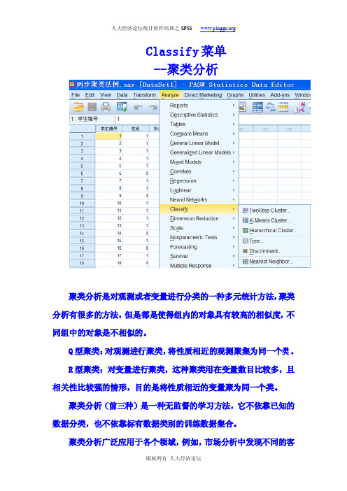
Classify菜单--聚类分析聚类分析是对观测或者变量进行分类的一种多元统计方法,聚类分析有很多的方法,但是都是使得组内的对象具有较高的相似度,不同组中的对象是不相似的。
Q型聚类:对观测进行聚类,将性质相近的观测聚集为同一个类。
R型聚类:对变量进行聚类,这种聚类用在变量数目比较多,且相关性比较强的情形,目的是将性质相近的变量聚为同一个类。
聚类分析(前三种)是一种无监督的学习方法,它不依靠已知的数据分类,也不依靠标有数据类别的训练数据集合。
聚类分析广泛应用于各个领域,例如,市场分析中发现不同的客户群,并且用不同的购买模式来刻画不同的客户群的特征。
SPSS中提供的聚类方法:1.two-step cluster-------两步聚类2.K-means cluster--------快速样本聚类过程3.Hierarchical cluster---分层聚类过程4.Tree--------------------决策树5.Discriminant------------判别分析6.Nearest neighbor--------最近邻分析第一讲:two-step cluster---两步聚类方法======================================================一:两步聚类法对数据的要求和特点二:两步聚类法原理三:噪声(noise)和局外者(outlier)的概念四:两步聚类法SPSS对话框介绍五:两步聚类法实例讲解和结果解释=======================================================一:两步聚类法的数据要求和特点:1.能同时处理连续变量和分类变量,两部聚类假设各变量是相互独立的,连续变量服从正态分布,分类变量服从多项式分布,但是参与分析的变量时常违反这些假设,但是两阶段估计仍然很好的作出估计。
2.可以根据指定的判别准则自动选择聚类的个数,也可以用户自己指定聚类个数,用户自己指定参数,叫做调谐(tuning),用户自已定义是依据BIC,Ratio of BIC Changes b、Ratio of Distance Measures c3.可以有效的分析大样本数据4.没有目标变量,只能对观测进行聚类5.在做两阶段聚类分析之前,可以先检验一下变量之间的独立性和变量的分布,SPSS提供的检验变量独立性的过程有:bivariz tecorr,crosstabs,means,检验变量正太性的过程有:explore,chi-squares,关于这些方法的应用,可以参考相关分析,descrip.菜单和非参数检验。

实验三SPSS统计分析与统计图表的绘制一、实验目的要求学生能够进行基本的统计分析;能够对频数分析、描述分析和探索分析的结果进行解读;完成基本的统计图表的绘制;并能够对统计图表进行编辑美化与结果分析;能够理解多元统计分析的操作(聚类分析和因子分析)。
二、实验内容与步骤2.1 基本的统计分析打开“分析/描述统计”菜单,可以看到以下几种常用的基本描述统计分析方法:1.Frequencies过程(频数分析)频数分析可以考察不同的数据出现的频数与频率,并且可以计算一系列的统计指标,包括百分位值、均值、中位数、众数、合计、偏度、峰度、标准差、方差、全距、最大值、最小值、均值的标准误等。
2.Descriptives过程(描述分析)调用此过程可对变量进行描述性统计分析,计算并列出一系列相应的统计指标,包括:均值、合计、标准差、方差、全距、最大值、最小值、均值的标准误、峰度、偏度等。
3.Explore过程(探索分析)调用此过程可对变量进行更为深入详尽的描述性统计分析,故称之为探索性统计。
它在一般描述性统计指标的基础上,增加有关数据其他特征的文字与图形描述,显得更加细致与全面,有助于用户思考对数据进行进一步分析的方案。
Descriptives:输出均数、中位数、众数、5%修正均数、标准误、方差、标准差、最小值、最大值、全距、四分位全距、峰度系数、峰度系数的标准误、偏度系数、偏度系数的标准误;Confidence Interval for Mean:平均值的%估计;M-estimators:作中心趋势的粗略最大似然确定,输出四个不同权重的最大似然确定数;Outliers:输出五个最大值与五个最小值;Percentiles:输出第5%、10%、25%、50%、75%、90%、95%位数。
4.Crosstabs过程(列联表分析)调用此过程可进行计数资料和某些等级资料的列联表分析,在分析中,可对二维至n维列联表(RC表)资料进行统计描述和χ2 检验,并计算相应的百分数指标。
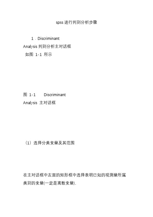
spss进行判别分析步骤1.DiscriminantAnalysis判别分析主对话框如图1-1 所示图1-1 DiscriminantAnalysis 主对话框(1)选择分类变量及其范围在主对话框中左面的矩形框中选择表明已知的观测量所属类别的变量(一定是离散变量),按上面的一个向右的箭头按钮,使该变量名移到右面的Grouping Variable 框中。
此时矩形框下面的Define Range按钮加亮,按该按钮屏幕显示一个小对话框如图1-2 所示,供指定该分类变量的数值范围。
图1-2 Define Range 对话框在Minimum 框中输入该分类变量的最小值在Maximum 框中输入该分类变量的最大值。
按Continue按钮返回主对话框。
(2)指定判别分析的自变量图1-3 展开SelectionVariable 对话框的主对话框在主对话框的左面的变量表中选择表明观测量特征的变量,按下面一个箭头按钮。
把选中的变量移到Independents 矩形框中,作为参与判别分析的变量。
(3)选择观测量图1-4 Set Value子对话框如果希望使用一部分观测量进行判别函数的推导而且有一个变量的某个值可以作为这些观测量的标识,则用Select 功能进行选择,操作方法是单击Select 按钮展开Selection Variable。
选择框如图1-3所示。
并从变量列表框中选择变量移入该框中再单击Selection Variable 选择框右侧的Value按钮,展开Set Value(子对话框)对话框,如图1-4 所示,键入标识参与分析的观测量所具有的该变量值,一般均使用数据文件中的所有合法观测量此步骤可以省略。
(4)选择分析方法在主对话框中自变量矩形框下面有两个选择项,被选中的方法前面的圆圈中加有黑点。
这两个选择项是用于选择判别分析方法的l Enterindependent together选项,当认为所有自变量都能对观测量特性提供丰富的信息时,使用该选择项。
层次聚类读书笔记值得注意的是,层次聚类方法是不可逆的,也就是说,当通过凝聚式的方法将两组合并后,无法通过分裂式的办法再将其分离到之前的状态,反之亦然。
另外,层次聚类过程中调查者必须决定聚类在什么时候停止,以得到某个数量的分类。
最后,必须记住,在不必要的情况下应该小心使用层次聚类方法。
最好用于有潜在层次结构的数据上。
凝聚式方法是层次聚类中被广泛使用的方法。
过程中,会产生一系列的分划:最初的是n 个单成员的类,最后的划分是一个包含全部个体的单个类。
凝聚式聚类有很多方法,但基本的操作是相似的,在每一步中,将距离最近的类或者个体融合成一个类。
方法之间的差异只是由不同的个体和组之间,或组与组之间的距离的计算方法而带来的。
下面介绍一些常用的方法。
单连锁(single linkage),又称最近邻(nearest neighbour)方法。
这个方法使用数据的相似度矩阵或距离矩阵,定义类间距离为两类之间数据的最小距离。
这个方法不考虑类结构。
可能产生散乱的分类,特别是在大数据集的情况下。
因为它可以产生chaining现象,当两类之间出现中间点的时候,这两类很有可能会被这个方法合成一类。
单连锁也可以用于分裂式聚类,用来分开最近邻距离最远的两组。
全连锁(complete linkage),又称最远邻(furthest neightbour)方法。
同样从相似度矩阵或距离矩阵出发,但定义距离为两类之间数据的最大距离。
同样不考虑到类的结构。
倾向于找到一些紧凑的分类。
(组)平均连锁(group average linkage),又称为UPGMA(Unweighted Pair-Group Methodusing the Average approach)。
跟前两个方法一样,从相似度矩阵或距离矩阵出发,但定义距离为类间数据两两距离的平均值。
这个方法倾向于合并差异小的两个类。
(距离)介于单连锁和全连锁之间。
它考虑到了类的结构,产生的分类具有相对的鲁棒性。
Stepwise Nearest Neighbor Discriminant Analysis∗Xipeng Qiu and Lide WuMedia Computing&Web Intelligence LabDepartment of Computer Science and EngineeringFudan University,Shanghai,Chinaxpqiu,ldwu@AbstractLinear Discriminant Analysis(LDA)is a popu-lar feature extraction technique in statistical pat-tern recognition.However,it often suffers fromthe small sample size problem when dealing withthe high dimensional data.Moreover,while LDAis guaranteed tofind the best directions when eachclass has a Gaussian density with a common co-variance matrix,it can fail if the class densitiesare more general.In this paper,a new nonpara-metric feature extraction method,stepwise nearestneighbor discriminant analysis(SNNDA),is pro-posed from the point of view of the nearest neigh-bor classification.SNNDAfinds the importantdiscriminant directions without assuming the classdensities belong to any particular parametric fam-ily.It does not depend on the nonsingularity of thewithin-class scatter matrix either.Our experimentalresults demonstrate that SNNDA outperforms theexisting variant LDA methods and the other state-of-art face recognition approaches on three datasetsfrom ATT and FERET face databases.1IntroductionThe curse of high-dimensionality is a major cause of thepractical limitations of many pattern recognition technolo-gies,such as text classification and object recognition.Inthe past several decades,many dimensionality reduction tech-niques have been proposed.Linear discriminant analysis(LDA)[Fukunaga,1990]is one of the most popular super-vised methods for linear dimensionality reduction.In manyapplications,LDA has been proven to be very powerful.The purpose of LDA is to maximize the between-class scat-ter while simultaneously minimizing the within-class scatter.It can be formulated by Fisher Criterion:J F(W)=W T S b WW T S w W,(1)where W is a linear transformation matrix,S b is the between-class scatter matrix and S w is the within-class scatter matrix.∗The support of NSF of China(69935010)and(60435020)is acknowledged.A major drawback of LDA is that it often suffers from the small sample size problem when dealing with the high dimen-sional data.When there are not enough training samples,S w may become singular,and it is difficult to compute the LDA vectors.For example,a100×100image in a face recog-nition system has10000dimensions,which requires more than10000training data to ensure that S w is nonsingular. Several approaches[Liu et al.,1992;Belhumeur et al.,1997; Chen et al.,2000;Yu and Yang,2001]have been proposed to address this problem.A common problem with all these proposed variant LDA approaches is that they all lose some discriminative information in the high dimensional space. Another disadvantage of LDA is that it assumes each class has a Gaussian density with a common covariance matrix. LDA guaranteed tofind the best directions when the distri-butions are unimodal and separated by the scatter of class means.However,if the class distributions are multimodal and share the same mean,it fails tofind the discriminant direction[Fukunaga,1990].Besides,the rank of S b is c−1, where c is the number of classes.So the number of extracted features is,at most,c−1.However,unless a posteriori prob-ability function are selected,c−1features are suboptimal in Bayes sense,although they are optimal with regard to Fisher criterion[Fukunaga,1990].In this paper,a new feature extraction method,step-wise nearest neighbor discriminant analysis(SNNDA),is pro-posed.SNNDA is a linear feature extraction method in or-der to optimize nearest neighbor classification(NN).Near-est neighbor classification[Duda et al.,2001]is an efficient method for performing nonparametric classification and of-ten used in the pattern classificationfield,especially in ob-ject recognition.Moreover,the NN classifier has a close relation with the Bayes classifier.However,when nearest neighbor classification is carried out in a high-dimensional feature space,the nearest neighbors of a point can be very far away,causing bias and degrading the performance of the rule[Hastie et al.,2001].Hastie and Tibshirani[Hastie and Tibshirani,1996]proposed a discriminant adaptive nearest neighbor(DANN)metric to stretch the neighborhood in the directions in which the class probabilities don’t change much, but their method also suffers from the small sample size prob-lem.SNNDA can be regarded as an extension of nonparametric discriminant analysis[Fukunaga and Mantock,1983],but itdoesn’t depend on the nonsingularity of the within-class scat-ter matrix.Moreover,SNNDAfinds the important discrimi-nant directions without assuming the class densities belong to any particular parametric family.The rest of the paper is organized as follows:Section2 gives the review and analysis of the current existing variant LDA methods.Then we describe stepwise nearest neighbor discriminant analysis in Section3.Experimental evaluations of our method,existing variant LDA methods and the other state-of-art face recognition approaches are presented in Sec-tion4.Finally,we give the conclusions in Section5.2Review and Analysis of Variant LDA MethodsThe purpose of LDA is to maximize the between-class scatter while simultaneously minimizing the within-class scatter. The between-class scatter matrix S b and the within-class scatter matrix S w are defined asS b=ci=1p i(m i−m)(m i−m)T(2)S w=ci=1p i S i,(3)where c is the number of classes;m i and p i are the mean vector and a priori probability of class i,respectively;m=ci=1p i m i is the total mean vector;S i is the covariance ma-trix of class i.LDA method tries tofind a set of projection vectors W∈R D×d maximizing the ratio of determinant of S b to S w,W=arg maxW |W T S b W||W T S w W|,(4)where D and d are the dimensionalities of the data before and after the transformation respectively.From Eq.(4),the transformation matrix W must be consti-tuted by the d eigenvectors of S−1w S b corresponding to itsfirstd largest eigenvalues[Fukunaga,1990].However,when the small sample size problem occurs,S wbecomes singular and S−1w does not exist.Moreover,if theclass distributions are multimodal or share the same mean(for example,the samples in(b),(c)and(d)of Figure2),it can fail tofind the discriminant direction[Fukunaga,1990].Many methods have been proposed for solving the above problems. In following subsections,we give more detailed review and analysis of these methods.2.1Methods Aimed at Singularity of S wIn recent years,many researchers have noticed the problem about singularity of S w and tried to overcome the computa-tional difficulty with LDA.To avoid the singularity of S w,a two-stage PCA+LDA ap-proach is used in[Belhumeur et al.,1997].PCA isfirst used to project the high dimensional face data into a low dimen-sional feature space.Then LDA is performed in the reduced PCA subspace,in which S w is non-singular.But this method is obviously suboptimal due to discarding much discrimina-tive information.Liu et al.[Liu et al.,1992]modified Fisher’s criterion by using the total scatter matrix S t=S b+S w as the denom-inator instead of S w.It has been proven that the modified criterion is exactly equivalent to Fisher criterion.However, when S w is singular,the modified criterion reaches the max-imum value,namely1,for any transformation W in the null space of S w.Thus the transformation W cannot guarantee the maximum class separability|W T S b W|is maximized.Be-sides,this method still needs to calculate an inverse matrix, which is time consuming.Chen et al.[Chen et al.,2000] suggested that the null space spanned by the eigenvectors of S w with zero eigenvalues contains the most discriminative in-formation.A LDA method(called NLDA)in the null space of S w was proposed.It chooses the projection vectors maximiz-ing S b with the constraint that S w is zero.But this approach discards the discriminative information outside the null space of S w.Figure1(a)shows that the null space of S w probably contains no discriminant information.Thus,it is obviously suboptimal because it maximizes the between-class scatter in the null space of S w instead of the original input space.Be-sides,the performance of the NLDA drops significantly when N−c is close to the dimension D,where N is the number of samples and c is the number of classes.The reason is that the dimensionality of the null space is too small in this situ-ation and too much information is lost[Li et al.,2003].Yu et al.[Yu and Yang,2001]proposed a direct LDA(DLDA) algorithm,whichfirst removes the null space of S b.They as-sume that no discriminative information exists in this space. Unfortunately,it be shown that this assumption is incorrect. Fig.1(b)demonstrates that the optimal discriminant vectors do not necessarily lie in the subspace spanned by the class centers.Figure1:(a)shows that the discriminant vector(dashed line) of NLDA contains no discriminant information.(b)shows that the discriminant vector(dashed line)of DLDA is con-strained to pass through the two class centers m1and m2. But according to the Fisher criteria,the optimal discriminant projection should be solid line(both in(a)and(b)).2.2Methods Aimed at Limitations of S bWhen the class conditional densities are multimodal,the class separability represented by S b is poor.Especially in the case that each class shares the same mean,it fails tofind the dis-criminant direction because there is no scatter of the class means[Fukunaga,1990].Notice the rank of S b is c−1,so the number of extracted features is,at most,c−1.However,unless a posteriori prob-ability function are selected,c−1features are suboptimal in Bayes sense,although they are optimal with regard to Fisher criterion[Fukunaga,1990].In fact,if classification is the ultimate goal,we need only estimate the class density well near the decision boundary[Hastie et al.,2001].Fukunaga and Mantock[Fukunaga and Mantock,1983] presented a nonparametric discriminant analysis(NDA)in an attempt to overcome these limitations presented in LDA.In nonparametric discriminant analysis the between-class scat-ter S b is of nonparametric nature.This scatter matrix is gen-erally full rank,thus loosening the bound on extracted fea-ture dimensionality.Also,the nonparametric structure of this matrix inherently leads to the extracted features that preserve relevant structures for classification.Bressan et al.[Bressan and Vitri`a,2003]explored the nexus between nonparametric discriminant analysis(NDA)and the nearest neighbors(NN) classifier and gave a slight modification of NDA which ex-tends the two-class NDA to a multi-class version. Although these nonparametric methods overcomes the lim-itations of S b,they still depend on the singularity of S w(or ˆSw).The rank ofˆS w must be no more than N−c.3Stepwise Nearest Neighbor Discriminant AnalysisIn this section,we propose a new feature extraction method, stepwise nearest neighbor discriminant analysis(SNNDA). SNNDA also uses nonparametric between-class and within-class scatter matrix.But it does not depend on singularity of within-class scatter matrix and improves the performance of NN classifier.3.1Nearest Neighbor Discriminant AnalysisCriterionAssuming a multi-class problem with classesωi(i= 1,...,c),we define the extra-class nearest neighbor for a sample x∈ωi asx E={x /∈ωi|||x −x||≤||z−x||,∀z/∈ωi}.(5) In the same fashion,the set of intra-class nearest neighbors are defined asx I={x ∈ωi|||x −x||≤||z−x||,∀z∈ωi}.(6) The nonparametric extra-class and intra-class differences are defined as∆E=x−x E,(7)∆I=x−x I.(8) .The nonparametric between-class and within-class scatter matrix are defined asˆS b =Nn=1w n(∆E n)(∆E n)T,(9)ˆS w =Nn=1w n(∆I n)(∆I n)T,(10)where w n is the sample weight defined asw n=||∆I n||α||∆I n||α+||∆E n||α,(11)whereαis a control parameter between zero and infinity.Thissample weight is introduced to deemphasize the samples inthe class center and give emphases to the samples near to theother class.The sample that has a larger ratio between thenonparametric extra-class and intra-class differences is givenan undesirable influence on the scatter matrix.The sampleweights in Eq.(11)take values close to0.5near the classifica-tion boundaries and drop to zero as we move to class center.The control parameterαadjusts how fast this happens.In thispaper,we setα=6.From the Eq.(7)and(8),we can see that||∆E n||representsthe distance between the sample x n and its nearest neighborin the different classes,and||∆I n||represents the distance be-tween the sample x n and its nearest neighbor in the sameclass.Given a training sample x n,the accuracy of the nearestneighbor classification can be directly computed by examin-ing the differenceΘn=||∆E n||2−||∆I n||2,(12)where∆E and∆I are nonparametric extra-class and intra-class differences and defined in Eq.(7)and(8).If the differenceΘn is more than zero,x n will be correctlyclassified.Otherwise,x n will be classified to the false class.The larger the differenceΘn is,the more accurately the sam-ple x n is classified.Assuming that we extract features by the D×d linear pro-jection matrix W with a constraint that W T W is an identitymatrix,the projected sample x new=W T x.The projectednonparametric extra-class and intra-class differences can bewritten asδE=W T∆E andδI=W T∆I.So we expect tofind the optimal W to make the difference||δE n||2−||δI n||2inthe projected subspace as large as possible.W=arg maxWNn=1w n(||δE n||2−||δI n||2).(13)This optimization problem can be interpreted as:find thelinear transform that maximizes the distance between classes,while minimizing the expected distance among the samplesof a single class.Considering that,NXn=1w n(||δE n||2−||δI n||2)=NXn=1w n(W T∆E n)T(W T∆E n)−NXn=1w n(W T∆I n)T(W T∆I n)=tr(NXn=1w n(W T∆E n)(W T∆E n)T)−tr(NXn=1w n(W T∆I n)(W T∆I n)T)=tr(W T(NXn=1w n∆E n(∆E n)T)W)Figure2:First projected directions of NNDA(solid)and LDA(dashed)projections,for four artificial datasets.−tr(W T(NXn=1w n∆I n(∆I n)T)W)=tr(W TˆS b W)−tr(W TˆS w W)=tr(W T(ˆS b−ˆS w)W),(14) where tr(·)is the trace of matrix,ˆS b andˆS w are the non-parametric between-class and within-class scatter matrix,as defined in Eq.(9)and(10).So Eq.(13)is equivalent toW=arg maxWtr(W T(ˆS b−ˆS w)W).(15) We call Eq.(15)the nearest neighbor discriminant analysis criterion(NNDA).The projection matrix W must be constituted by the d eigenvectors of(ˆS b−ˆS w)corresponding to itsfirst d largest eigenvalues.Figure2gives comparisons between NNDA and LDA. When the class density is unimodal((a)),NNDA is approxi-mately equivalent to LDA.But in the cases that the class den-sity is multimodal or that all the classes share the same mean ((b),(c)and(d)),NNDA outperforms LDA greatly.3.2Stepwise Dimensionality ReductionIn the analysis of the nearest neighbor discriminant analysis criterion,notice that we calculate nonparametric extra-class and intra-class differences(∆E and∆I)in original high di-mensional space,then project them to the low dimensional space(δE=W T∆E andδI=W T∆I),which does not ex-actly agree with the nonparametric extra-class and intra-class differences in projection subspace except for the orthonor-mal transformation case,so we have no warranty on distance preservation.A solution for this problem is tofind the projec-tion matrix W by stepwise dimensionality reduction method. In each step,we re-calculate the nonparametric extra-class and intra-class differences in its current dimensionality.Thus, we keep the consistency of the nonparametric extra-class and intra-class differences in the process of dimensionality reduc-tion.Figure3gives the algorithm of stepwise nearest neighbor discriminant analysis.•Give D dimensional samples{x1,···,x N},we expect tofind d dimensional discriminant subspace.•Suppose that wefind the projection matrix W via Tsteps,we reduce the dimensionality of samples to d t in step t,and d t meet the conditions:d t−1>d t>d t+1, d0=D and d T=d.•For t=1,···,T1.Calculate the nonparametric between-classˆS tband within-class scatter matrixˆS t w in the current d t−1dimensionality,2.Calculate the projection matrix W t, W t is d t−1×d tmatrix.3.Project the samples by the projection matrix W t,x= W T t×x.•Thefinal transformation matrix W=Tt=1Wt. Figure3:Stepwise Nearest Neighbor Discriminant Analysis3.3DiscussionsSNNDA has an advantage that there is no need to calculate the inverse matrix,so it is a more efficient and stable method. Moreover,though SNNDA optimizes the1-NN classification, it is easy to extend it to the case of k-NN.However,a drawback of SNNDA is the computational in-efficiency infinding the neighbors when the original data space is high dimensionality.A improved method is that PCA isfirst used to reduce the dimension of data to N−1(the rank of the total scatter matrix)through removing the null space of the total scatter matrix.Then,SNNDA is performed in the transformed space.Yang et al.[Yang and Yang,2003]shows that no discriminant information is lost in this transformed space.4ExperimentsIn this section,we apply our method to face recognition and compare it with the existing variant LDA methods and the other state-of-art face recognition approaches,such as PCA[Turk and Pentland,1991],PCA+LDA[Belhumeur et al.,1997],NLDA[Chen et al.,2000],NDA[Bressan and Vitri`a,2003]and Bayesian[Moghaddam et al.,2000]ap-proaches.All the experiments are repeated5times indepen-dently and the average results are calculated.4.1DatasetsTo evaluate the robustness of SNNDA,we perform the ex-periments on three datasets from the popular ATT facedatabase[Samaria and Harter,1994]and FERET face database[Phillips et al.,1998].The descriptions of the three datasets are below:ATT Dataset This dataset is the ATT face database(for-merly‘The ORL Database of Faces’),which con-tains400images(112×92)of40persons,10im-ages per person.The images are taken at differ-ent times,varying lighting slightly,facial expres-sions(open/closed eyes,smiling/non-smiling)and fa-cial details(glasses/no-glasses).Each image is linearly stretched to the full range of pixel values of[0,255].Fig.4shows some face examples in this database.The set of the10images for each person is randomly parti-tioned into a training subset of5images and a test set of the other5.The training set is then used to learn basis components,and the test set forevaluate.Figure4:Face examples from ATT databaseFERET Dataset1This dataset is a subset of the FERETdatabase with194subjects only.Each subject has3images:(a)one taken under controlled lighting condi-tion with a neutral expression;(b)one taken under thesame lighting condition as above but with different fa-cial expressions(mostly smiling);and(c)one taken un-der different lighting condition and mostly with a neutralexpression.All images are pre-processed using zero-mean-unit-variance operation and manually registeredusing the eye positions.All the images are normal-ized by the eye locations and are cropped to the size of75×65.A mask template is used to remove the back-ground and the hair.Histogram equalization is appliedto the face images for photometric normalization.Twoimages for each person is randomly selected for trainingand the rest one is used for test.FERET Dataset2This dataset is a different subset of theFERET database.All the1195people from the FERETFa/Fb data set are used in the experiment.There aretwo face images for each person.This dataset has nooverlap between the training set and the galley/probe setaccording to the FERET protocol[Phillips et al.,1998].500people are randomly selected for training,and theremaining695people are used for testing.For each test-ing people,one face image is in the gallery and the otheris for probe.All images are pre-processed by using thesame method in FERET Dataset1.4.2Experimental ResultsFig.5shows the rank-1recognition rates with the differentnumber of features on the three different datasets.It is shownthat SNNDA outperforms the other methods.The recogni-tion rate of SNNDA can reach almost100%on ATT dataset.The recognition rate of SNNDA have reached100%on twoFERET dataset surprisedly when the dimensionality of sam-ples is about20,while the other methods have poor perfor-mances in the same dimensionality.Moreover,SNNDA doesnot suffer from overfitting.Except SNNDA and PCA,therank-1recognition rates of the other methods have a descentwhen the dimensionality increases continuously.Fig.6shows cumulative recognition rates on the three dif-ferent datasets.From it,we can see that none of the cumula-tive recognition rates can reach100%except SNNDA.When dataset contains the changes of lighting condition(such as FERET Dataset1),SNNDA also has obviously bet-ter performance than the others.Different from ATT dataset and FERET dataset1,wherethe class labels involved in training and testing are the same,the FERER dataset2has no overlap between the trainingset and the galley/probe set according to the FERET proto-col[Phillips et al.,1998].The ability of generalization fromknown subjects in the training set to unknown subjects in thegallery/probe set is needed for each method.Thus,the resulton FERET dataset2is more convincing to evaluate the robustof each method.We can see that SNNDA also gives the bestperformance than the other methods on FERET dataset2.A major character,displayed by the experimental results,is that SNNDA always has a stable and high recognition rateson the three different datasets,while the other methods haveunstable performances.5ConclusionIn this paper,we proposed a new feature extraction method,stepwise nearest neighbor discriminant analysis(SNNDA),whichfinds the important discriminant directions without as-suming the class densities belong to any particular paramet-ric family.It does not depend on the nonsingularity of thewithin-class scatter matrix either.Our experimental resultson the three datasets from ATT and FERET face databasesdemonstrate that SNNDA outperforms the existing variantLDA methods and the other state-of-art face recognition ap-proaches greatly.Moreover,SNNDA is very efficient,accu-rate and robust.In the further works,we will extend SNNDAto non-linear discriminant analysis with the kernel method.Another attempt is to extend SNNDA to the k-NN case.References[Belhumeur et al.,1997]P.N.Belhumeur,J.Hespanda,andD.Kiregeman.Eigenfaces vs.Fisherfaces:Recognitionusing class specific linear projection.IEEE Transactionson Pattern Analysis and Machine Intelligence,19(7):711–720,1997.[Bressan and Vitri`a,2003]M.Bressan and J.Vitri`a.Nonparametric discriminant analysis and nearestneighbor classification.Pattern Recognition Letters,24:2743C2749,2003.[Chen et al.,2000]L.Chen,H.Liao,M.Ko,J.Lin,andG.Yu.A new LDA-based face recognition system whichcan solve the small sample size problem.Pattern Recog-nition,33(10):1713–1726,2000.Number of features R e c o g n i t i o n r a t e sNumber of features R e c o g n i t i o n r a t e sNumber of featuresR e c o g n i t i o n r a t e sFigure 5:Rank-1recognition rates with the different number of features on the three different datasets.(Left:ATT dataset;Middle:FERET dataset 1;Right:FERET dataset 2)Rank R e c o g n i t i o n r a t e sRank R e c o g n i t i o n r a t e sRankR e c o g n i t i o n r a t e sFigure 6:Cumulative recognition rates on the three different datasets.Left:ATT dataset(the number of features is 39;Mid-dle:FERET dataset 1(the number of features is 60);Right:FERET dataset 2(the number of features is 60)[Duda et al.,2001]R.O.Duda,P.E.Hart,and D.G.Stork.Pattern classification .Wiley,New York,2nd edition,2001.[Fukunaga and Mantock,1983]K.Fukunaga and J.Man-tock.Nonparametric discriminant analysis.IEEE Trans-actions on Pattern Analysis and Machine Intelligence ,5:671C678,1983.[Fukunaga,1990]K.Fukunaga.Introduction to statistical pattern recognition .Academic Press,Boston,2nd edition,1990.[Hastie and Tibshirani,1996]T.Hastie and R.Tibshirani.Discriminant adaptive nearest neighbor classification.IEEE Transactions on Pattern Analysis and Machine In-telligence ,18:607C616,1996.[Hastie et al.,2001]T.Hastie,R.Tibshirani,and J.Fried-man.The Elements of Statistical Learning .Springer,New York,2001.[Li et al.,2003]H.F.Li,T.Jiang,and K.S.Zhang.Efficient and robust feature extraction by maximum margin crite-rion.In Proc.of Neural Information Processing Systems ,2003.[Liu et al.,1992]K.Liu,Y .Cheng,and J.Yang.A general-ized optimal set of discriminant vectors.Pattern Recogni-tion ,25(7):731C739,1992.[Moghaddam et al.,2000]B.Moghaddam,T.Jebara,and A.Pentland.Bayesian face recognition.Pattern Recog-nition ,33:1771–1782,2000.[Phillips et al.,1998]P.J.Phillips,H.Wechsler,J.Huang,and P.Rauss.The feret database and evaluation proce-dure for face recognition algorithms.Image and Vision Computing ,16(5):295–306,1998.[Samaria and Harter,1994]Ferdinando Samaria and Andy Harter.Parameterisation of a stochastic model for human face identification.In Proc.of 2nd IEEE Workshop on Ap-plications of Computer Vision ,1994.[Turk and Pentland,1991]M.Turk and A.Pentland.Eigen-faces for recognition.Journal of Cognitive Neuroscience ,3(1):71–86,1991.[Yang and Yang,2003]J.Yang and J.Y .Yang.Why can LDA be performed in PCA transformed space?Pattern Recognition ,36:563–566,2003.[Yu and Yang,2001]H.Yu and J.Yang.A direct LDA al-gorithm for high-dimensional data with application to face recognition.Pattern Recognition ,34:2067–2070,2001.。