SolverChange函数

Excel Solver(3)：求解步骤和数据组织作者：XLFinance 来源：XLFinance 打印邮寄返回求解的一般步骤使用Excel规划求解工具解决优化问题的基本步骤包括：1）识别问题，明确优化方程模型2）组织数据3）确定模型决策变量所在单元格Solver在求解问题过程中会不断调整决策变量的取值可变单元格的数量不能超过200个使用引用单元格、命名或区域识别可变单元格必须位于活动的工作表上4）确定包含Excel公式（代表依赖于决策变量的目标函数）的目标单元格：目标单元格必须是引用单元格或一个区域名称目标单元格在多数情况下应包含公式必须指定求解的目标为最大值、最小值或一个指定的数值5）确定模型约束条件6）通过规划求解工具实施正如上文对局部最优和全局最优的解释，不同的初始值可能导致不同的求解结果。

复杂的非线性问题中，在识别问题和组织数据阶段可能还需要对问题的预分析，确定适当的决策变量初始值。

运行过程和结果报告求解运行Solver后，Solver会处于求解状态直至：找到一个方案；确定无法找到解决方案；运行时间超出最高限制；找到最优解如找到最优解，则Solver将返回对话框，提示用户选择下一步的操作。

可选择的操作包括：将Solver的求解结果写入可变单元格区域或放弃Solver求解结果，将可变单元格恢复至原始值状态。

Solver返回的最优解结果可能包括以下不同的类型：可行解：满足所有的约束，但如有可能，Solver会继续求解更优的解；局部最优：在初始值的“邻近地带”没有找到更好的解决方案；全局最优：不存在更好的解决方案；无法找到解决方案有多个原因可能导致Solver无法求解，其中部分是计算原因，部分则是操作原因，如为后者则应根据提示错误信息进行相应调整。

结果报告在规划求解结果对话框中可以选择输出的报告类型，其中包括：求解报告、敏感性报告和极值报告三种。

Solver会自动添加相关工作表并命名。

求解报告是对求解结果的综述，包括目标单元格和可变单元格的初始值和最终值、约束及相关信息。

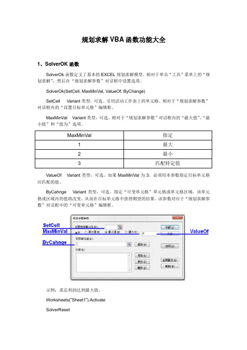
规划求解VBA函数功能大全1、SolverOK函数SolverOk函数定义了基本的EXCEL规划求解模型。

相对于单击“工具”菜单上的“规划求解”，然后在“规划求解参数”对话框中设置选项。

SolverOk(SetCell, MaxMinVal, ValueOf, ByChange)SetCell Variant类型，可选。

引用活动工作表上的单元格。

相对于“规划求解参数”对话框内的“设置目标单元格”编辑框。

MaxMinVal Variant类型，可选。

相对于“规划求解参数”对话框内的“最大值”、“最小值”和“值为”选项。

MaxMinVal 指定1 最大2 最小3 匹配特定值ValueOf Variant类型，可选。

如果MaxMinVal为3，必须用本参数指定目标单元格应匹配的值。

ByCahnge Variant类型，可选。

指定“可变单元格”单元格或单元格区域，该单元格或区域内的值将改变，从而在目标单元格中获得期望的结果。

该参数对应于“规划求解参数”对话框中的“可变单元格”编辑框。

示例：求总利润达到最大值。

Worksheets(“Sheet1”).ActivateSolverResetSolverOption Precision:=0.001SolverOK setCell:=Range(‘TotalProfit”), _MaxMinVal:=1, _ByChange:=Range(“C4:E6”)SolverAdd CellRef:=Range(“F4:F6”), _Relation:=1, _FormulaT ext:=100SolverAdd CellRef:=Range(“C4:E6”), _Relation:=3, _FormulaT ext:=0SolverAdd CellRef:=Range(“C4:E6”), _Relation:=4SolverSolve UserFinish:=FalseSolverSave SaveArea:=Range(“A33”)2、SoverReset函数重新设置“规划求解参数”对话框中的所有单元格选定区域和约束条件，并将“规划求解选项”对话框中的所有设定恢复为默认值。

Microsoft Excel 规划求解的说明Microsoft Excel 规划求解是一个Microsoft Excel Add-in Microsoft Excel Solver 有助于您确定Microsoft Excel 工作表上的特定目标单元格中公式的最优值。

Microsoft Excel 规划求解调整其他单元格使用的公式与目标单元格的值。

在构建一个公式，并定义公式中的参数或变量的约束的一组后，Microsoft Excel 规划求解尝试到达满足所有约束的应答的各种解决方案。

Microsoft Excel 规划求解使用下列元素来"解决公式：∙目标单元格的程序的目标单元格的目标。

它是在工作表模型将最小化、最大化，或设置为特定值的单元格。

∙更改单元格的Changing 单元格为决策变量。

这些单元格会影响目标单元格的值。

这些单元格更改Microsoft Excel 规划求解查找目标单元格的最佳解决方案。

∙约束的约束是限制内容的单元格。

是例如尽管另一个单元格可能限制为在给定的值小于，可能限制为整数的值工作表模型中的一个单元格。

可以通过使用Microsoft Visual Basic for Applications (VBA) 宏自动执行创建和Microsoft Excel 规划求解模型的操作。

本文介绍如何使用VBA 宏语言在Microsoft Excel 97 中使用Microsoft Excel 规划求解函数。

本文假定您熟悉VBA 语言和用于Microsoft Excel 97，Microsoft Visual Basic 编辑器。

本文中使用的示例有以下Microsoft Web 站点下载：/download/excel97win/solverex/1.0/WIN98Me/EN-US/ SolverEx.exe请注意您还可以在宏和Microsoft Excel 版本 5.0 和7.0 中的本文所述的示例。

HP 35s Using the formula solver – part 2Overview of the formula solverPractice Example: A formula with several variables Practice Example: A direct solutionPractice Example: Where two functions intersectOverview of the Formula SolverGiven an expression of the form:f(x) = yThe HP Solve Application searches for a value of x that gives:f(x) = y = 0A value of x for which this is true is called a root, and it provides a solution of the equation f(x) = 0. The graph in Figure 1 shows this graphically – there is a root at the value of x where f(x) is zero.1FigureOn the HP 35s, f(x) can be typed as a formula, in equation mode, or it can be typed as a program. When the Solver is used to find a root of a formula or equation typed in equation mode, it is referred to as the Formula Solver.Part 1 of this training aid provided an introduction to the Formula Solver, using a few simple examples. This second part explains how the Solver works, and shows some more examples.The Formula Solver works with f(x) as a formula containing x, for example3x² - 3x - 15 or 5sin(x) – 7log(x)If the Formula Solver is given an equation with terms on both sides of the equals sign, such as:3x² + 4x = 7x +15then it begins by moving everything to one side of the equals sign, so the above equation would become the formula:f(x) = 3x² - 3x - 15 = 0The Formula Solver ignores the = 0 part, as it is trying to find a value for x to make the formula zero. So there is no need to type an equation with = 0 in it; it is enough to type the formula.The variable x in the above is called the unknown variable. It can be represented by any of the HP 35s variables A through Z. A formula can contain more than one variable, the Solver will ask which is the unknown variable and will then ask for the known values of all the other variables.The Formula Solver then tries to rearrange the equation f(x) = 0 to give a direct solution for x. An example will be shown later.If a direct solution is not found, the Solver begins by first trying two guesses for the unknown variable. The user can give one or two guesses for the Solver to start from. The first part showed that this can be very useful, either to direct the Solver towards one root of several, or to direct the Solver away from values that would cause an error. Good guesses can also speed up the search for a root. In some cases the function varies very slowly over some values, and a good guess is needed to direct the Solver away from them and towards the range of values where a solution is expected. Beginning from the values obtained for the first two guesses, the Solver searches for values of the unknown variable that make f(x) smaller. If two guesses have the opposite sign, the Solver tries to narrow down the region between them until it finds where the sign changes and f(x) is zero. If two guesses have the same sign, the Solver uses the difference between them to pick the direction in which to change x to look for a third value closer to zero.The process is repeated until one of the following happens.A value of x is found for which f(x) is exactly zero.Two neighboring values of x are found, differing by 1 or 2 in the twelfth significant digit, such that f(x) changes sign between them. An example of this was given in part 1.No value can be found, but the Solver finds a minimum. An example was given in part 1.No value can be found because the Solver is looking at values of x for which f(x) is constant.No value can be found because f(x) is decreasing asymptotically towards a non-zero value.Two more cases arise because the HP 35s works with a finite range of numbers, negative numbers between-10500 and -10-499, 0 and positive numbers between +10-499 and +10500. This range is sufficient to cover allphysical measurements, and even all numbers in government finances, but problems in number theory and in combinatorial operations may require numbers outside this range. (To be exact, the largest absolute value that the HP 35s can work with is 9.99999999999E499.)No value can be found because the root is at a value of x that is not zero but lies between -10-499 and +10-499. In such a case the Solver gives a result of 0.No value can be found because the root is at x that is more negative than, or equal to, -10500 or greater than or equal to +10500 . In such a case the Solver stops with an OVERFLOW error.To help the user distinguish between the above, the Solver returns the last value it tried for x, the last but one value tried, and the value of f(x) at the last value. Part 1 showed how these values can be seen in RPN mode and in Algebraic mode.The following examples show some of the features that were not included in part 1.Practice Example: A formula with several variablesExample 1: A factory is to produce tin cans with a volume of 100 cubic centimeters. The designer estimates that the height should be 10 cm and the radius about 2 cm. Calculate the exact volume of this can, and if it is notclose to 100 cubic centimeters then recalculate the radius to give the required volume.Solution: The equation for a cylinder’s volume V, given its radius r, and height h, is V = π r² h. Enter this as the formula π r² h – V in equation mode and then use the Solver.Go to equation mode by typing d. If necessary, put the new equation in a particular place in the list ofequations by moving up or down through the list with the up and down cursor keys below the HP 35sscreen.Enter the formula by typing:¹j¸hR)2¸hHÃhVÏAs was explained in part 1, to enter a variable into an equation, press the h key and then one of theletter keys. As with ºe, the symbol A..Z at the top of the screen is shown as a reminder that one ofthe keys marked A through Z must be pressed. For example press the 5 key to enter the variable V.2FigureTo solve the equation, press the ºÛ key. The Solver asks which variable to solve for:Figure3The symbol A..Z is at the top of the screen again. The variable in this formula is V so press 5 again. TheSolver now knows that V is the unknown variable and it asks for the values of the known variables.Figure4The value that is already stored in R is shown too. If this is the required value then it is enough to press¥. If the variable R has not been used before, then its value is zero. In this example, type the radius 2and press ¥.5FigureThe Solver asks for the other known variable. Type the height, 10, and press ¥ again. The HP 35sdisplays SOLVING for a moment, then the result.6FigureThe volume is over 125 cubic centimeters, considerably more than the intended 100. Repeat thecalculation, but this time use the known volume of 100, and solve for the radius. Solve the equation againby pressing dºÛ. The Solver asks for the unknown variable, press R. The Solver then asksfor the known variables, first H.7FigureThe present value of H is the value previously given. As this is to remain the same, just press ¥ again.The Solver now asks for the other variable, V.8FigureThe present value of V is shown; this is the volume just calculated. As the volume should be 100, type 100and press ¥. The Solver calculates and displays the radius needed to give the required volume.9FigureAnswer: The cans should have a radius of 1.78 cm.Practice Example: A direct solutionExample 2: To show that the HP 35s looks for a direct solution before starting to search for a root, try to solve ln(z) = 0 beginning from a negative number for the guess.Solution: Store –5 in Z. Then store LN(z) as the formula to solve. This means that a solution is wanted for the equation LN(z) = 0.5zºeZdº&hZÏ10FigureTo solve the equation, press ºÛZ. The Solver immediately displays the answer:11FigureAnswer: Z = 1 is the solution to LN(z) = 0. This is obvious, the point of this example is that the answer was found immediately, and the negative guess was not tried. If the negative guess had been tried, it would havecaused a LOG(NEG) error, as in Example 3 of part 1. The Formula Solver recognized that Z appears onlyonce in the formula, and that LN(Z) = 0 can therefore be rewritten as Z = exp(0) to solve for Z directly. Suchdirect solutions can speed up the use of Solver, specially when a complicated formula with severalvariables is being solved several times for different variables.Note: Where more than one solution is possible, for example ASIN(Y)=0, the direct solution is the “principal” value. For example, for ASIN(Y)=0, this is 0 degrees, not 180 degrees, or –180 degrees, or any other possible value. In the same way, an equation such as X²=4 is solved directly and returns the positive root 2. To find other roots, it is necessary to write the expression in such a way that the Solver does not find a direct solution. An easy way to achieve this is to add 0× the unknown variable into an expression, for example ASIN(Y) + 0×Y = 0 or X² + 0×X = 0. This is because the Solver stops looking for a direct solution as soon as it sees the unknown variable more than once in an expression.Practice Example: Where two functions intersectThe Formula Solver can also be used to solve problems of the form:g(x) = h(x)This requires a value of x at which one function g(x) is equal to another function h(x). In other words, the problem is to find x at which these functions intersect.The equation can be rewritten as:f(x) = g(x) - h(x) = 0Solving the formula g(x) – h(x) will give the value of x at which the two functions cross over.Example 3: The factory from Example 1 is interested in designing spherical containers with the same volume and the same radius as their tin cans. This means that they want to find a radius r such that:V = π r² h = 4/3 π r³Solution: Modify the formula from Example 1 to find r such that π r² h – 4/3 π r³ is zero.A quick look at this expression shows that one solution is r = 0. This is not a useful solution so it would behelpful to provide a guess to direct the Solver away from zero. One guess is the value already in R. Type 8on the lower line of the display as the second guess.Go to equation mode by typing d. Find the old equation by moving up or down through the equation listwith the × and Ø keys.Begin editing the formula by pressing the left cursor key Ö. The cursor appears at the end of the formula.12Figure~ to delete the V. Then type the formula for the volume of a sphere.Press4¯3¸¹j¸hR)3ÏPress the right-arrow Õ key a few times to see the last part of the changed formula. It should look as inFigure 13.Figure13To solve the equation, press the Û key. The Solver asks which variable to solve for: The unknownvariable is R so press R. The Solver now asks for the value of the known variable H.14FigureThis value is to stay unchanged, so press ¥. The Solver looks for a solution.15FigureAnswer: If both the radius of the sphere and that of the base of the cylindrical can are 7.5 then the sphere and the can will have the same volume.The Solver can be used for many kinds of problems, further information is given in the HP 35s manual, and a detailed description of the Solver is provided in Appendix D of the manual.。

如何在Excel中使用Solver进行优化问题求解Excel中的Solver是一种强大的工具，可以帮助我们解决优化问题。

无论是在学习、工作还是日常生活中，我们都会遇到一些需要在给定的条件下寻找最优解的情况。

本文将介绍如何在Excel中使用Solver进行优化问题求解。

1. 引言优化问题是数学和工程领域中常见的问题。

在很多情况下，我们需要找到一个最优解，使得满足一定的条件，并使目标函数值最大或最小化。

在Excel中使用Solver工具可以帮助我们自动寻找最优解，而无需手动尝试不同的解决方案。

2. 准备工作在开始使用Solver之前，我们首先需要在Excel中安装和启用Solver插件。

在Excel 2010及以上版本中，我们可以通过以下步骤来启用Solver插件：a. 点击Excel菜单中的“文件”选项；b. 选择“选项”；c. 在弹出的对话框中选择“加载项”；d. 在加载项管理器中，勾选“Solver插件”；e. 点击“确定”按钮，完成插件的启用。

3. 设置优化问题在Excel中，我们通常将优化问题建模为一个规划问题。

我们需要明确定义目标函数、约束条件和可调整的变量。

（下面仅以线性规划问题为例，后续也可适用于非线性规划问题。

）目标函数：我们首先需要明确我们的优化目标是什么，是最大化还是最小化。

在Excel中，我们可以利用单元格来表示目标函数，并将其命名为目标函数。

约束条件：我们需要确保我们的解决方案满足一定的条件。

这些条件可以是等式、不等式或者其他限制条件。

同样地，在Excel中，我们可以使用单元格来表示约束条件，并将其命名为约束条件。

可调整的变量：我们需要确定哪些变量是可调整的，它们是我们希望Solver来求解的。

在Excel中，我们可以使用单元格来表示这些可调整的变量，并将其命名为变量。

4. 使用Solver求解问题在完成优化问题的设置后，我们可以开始使用Solver来求解问题了。

我们可以按照以下步骤进行操作：a. 点击Excel菜单中的“数据”选项；b. 在数据选项中，找到“分析”工具，点击打开；c. 在弹出的对话框中选择“Solver”；d. 在Solver对话框中，我们需要对一些设置进行配置：- 设置目标单元格为我们定义的目标函数单元格；- 设置可调整单元格为我们定义的变量单元格；- 设置约束条件为我们定义的约束条件单元格；- 设置约束条件的限制类型，可以是等式、不等式或者其他限制条件；- 如果有需要，我们还可以设置其他选项，如求解方法、可行域还是全局解等；e. 点击“求解”按钮，Solver将自动寻找最优解，并将结果显示在Excel中。

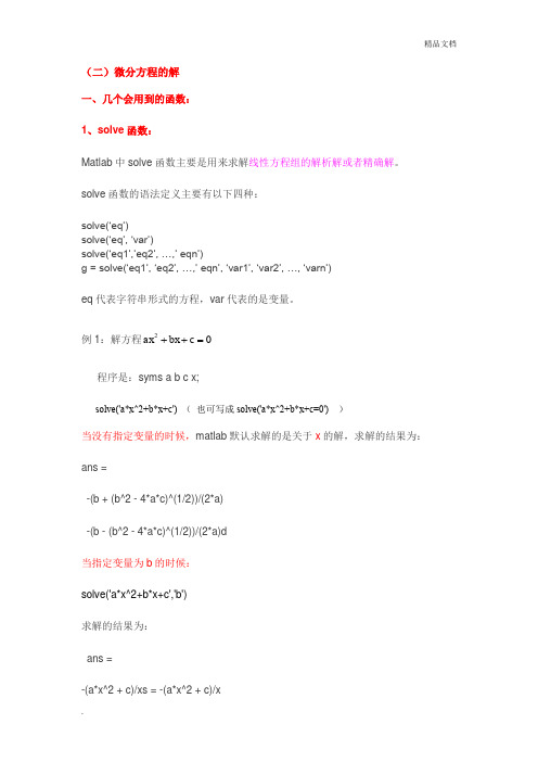
（二）微分方程的解 一、几个会用到的函数：1、solve 函数：Matlab 中solve 函数主要是用来求解线性方程组的解析解或者精确解。

solve 函数的语法定义主要有以下四种：solve(‘eq’)solve(‘eq’, ‘var’)solve(‘eq1’,’eq2’, …,’ eqn’)g = solve(‘eq1’, ‘eq2’, …,’ eqn’, ‘var1’, ‘var2’, …, ‘varn’)eq 代表字符串形式的方程，var 代表的是变量。

例1：解方程02=++c bx ax程序是：syms a b c x;solve('a*x^2+b*x+c') （ 也可写成solve('a*x^2+b*x+c=0') ）当没有指定变量的时候，matlab 默认求解的是关于x 的解，求解的结果为： ans =-(b + (b^2 - 4*a*c)^(1/2))/(2*a)-(b - (b^2 - 4*a*c)^(1/2))/(2*a)d当指定变量为b 的时候：solve('a*x^2+b*x+c','b')求解的结果为：ans =-(a*x^2 + c)/xs = -(a*x^2 + c)/x例2：对于方程组⎩⎨⎧=-=+5111y x y x 的情况S=solve('x+y=1','x-11*y=5');S.xS.y>> S=[S.x,S.y](这里或者写成x=S.x y=S.y) 如果解得是一个方程组，而且采用了形如[a,b]=solve(a+b=1, 2a-b=4ab) 的格式，那么，在MATLAB R2014a 中没问题，可以保证输出的a ，b 就等于相应的解，但是在R2012b 等早先版本中不能保证输出的顺序就是你声明变量时的顺序。

所以最好采用g=solve(a+b=1, 2a-b=4ab)这种单输出格式，这样输出的是一个结构体，g.a 和g.b 就是对应的解。

Excel的Solver功能的应用技巧Excel是一款功能强大的电子表格软件，它不仅可以处理大量数据，还具备多种工具和功能，如图表制作、数据分析和预测。

其中，Solver功能是Excel中一个非常有用的工具，它可以帮助我们解决各种复杂的问题，并找到最佳的方案。

本文将介绍Solver功能的应用技巧，帮助读者更好地利用Excel解决实际问题。

1. Solver功能简介Solver是Excel的一种附加组件，它主要用于求解优化问题。

通过设置目标单元格、约束条件和可变单元格，Solver可以自动计算出最优的结果，使目标单元格的值最大或最小。

Solver可以解决线性优化问题和非线性优化问题，对于复杂的多元非线性方程组，也可以进行求解。

2. 使用Solver解决线性规划问题线性规划是一种优化问题，目标函数和约束条件都是线性的。

对于这种问题，我们可以使用Solver功能来找到最优解。

首先，我们需要将问题转化为线性规划模型，然后在excel中输入目标函数和约束条件，并设置好目标单元格和可变单元格。

接下来，打开Solver对话框，选择目标单元格、最大化或最小化目标值，以及约束条件，之后运行Solver，它将自动计算出最佳的解决方案。

3. 使用Solver解决非线性规划问题非线性规划问题是指目标函数或约束条件中存在非线性关系的问题。

对于这种问题，我们可以通过使用Solver的非线性求解功能来找到最优解。

在excel中输入目标函数和约束条件，并设置好目标单元格和可变单元格，然后打开Solver对话框，选择目标单元格、最大化或最小化目标值，以及约束条件。

此时，需要注意选择Solver引擎为“GRG Nonlinear”，该引擎可以处理非线性问题。

运行Solver后，它将自动进行迭代计算，并给出最佳解。

4. 使用Solver进行参数优化除了解决规划问题，Solver还可以用于参数优化。

通过改变某些参数的取值，我们可以获得不同的结果。

sklearn神经⽹络MLPclassifier参数详解参数备注hidden_l ayer_sizes tuple，length = n_layers - 2，默认值（100，）第i个元素表⽰第i个隐藏层中的神经元数量。

激活{‘identity’，‘logistic’，‘tanh’，‘relu’}，默认’relu’ 隐藏层的激活函数：‘identity’，⽆操作激活，对实现线性瓶颈很有⽤，返回f（x）= x；‘logistic’，logistic sigmoid函数，返回f（x）= 1 /（1 + exp（-x））；‘tanh’，双曲tan函数，返回f（x）= tanh（x）；‘relu’，整流后的线性单位函数，返回f（x）= max（0，x）slover {‘lbfgs’，‘sgd’，‘adam’}，默认’adam’。

权重优化的求解器：'lbfgs’是准⽜顿⽅法族的优化器；'sgd’指的是随机梯度下降。

'adam’是指由Kingma，Diederik和Jimmy Ba提出的基于随机梯度的优化器。

注意：默认解算器“adam”在相对较⼤的数据集（包含数千个训练样本或更多）⽅⾯在训练时间和验证分数⽅⾯都能很好地⼯作。

但是，对于⼩型数据集，“lbfgs”可以更快地收敛并且表现更好。

alpha float，可选，默认为0.0001。

L2惩罚（正则化项）参数。

batch_size int，optional，默认’auto’。

⽤于随机优化器的minibatch的⼤⼩。

如果slover是’lbfgs’，则分类器将不使⽤minibatch。

设置为“auto”时，batch_size = min（200，n_samples）learning_rate {‘常数’，‘invscaling’，‘⾃适应’}，默认’常数"。

⽤于权重更新。

仅在solver ='sgd’时使⽤。

'constant’是’learning_rate_init’给出的恒定学习率；'invscaling’使⽤’power_t’的逆缩放指数在每个时间步’t’逐渐降低学习速率learning_rate_， effective_learning_rate = learning_rate_init / pow（t，power_t）；只要训练损失不断减少，“adaptive”将学习速率保持为“learning_rate_init”。

一、prepareGeometryChange函数概述在Qt框架中，prepareGeometryChange函数是一个用于准备改变对象的几何属性的重要函数。

这个函数通常被用于在改变一个对象的几何属性之前，做一些准备工作，以确保对象的几何属性能够被正确地改变。

这个函数的使用对于保证对象的几何属性的正确性和一致性非常重要。

二、prepareGeometryChange函数的参数prepareGeometryChange函数通常会接受一些参数，以便对对象的几何属性做出相应的准备工作。

这些参数可能包括但不限于：1. QRectF rect：表示要改变的对象的几何矩形，用来描述对象的位置和大小。

2. QRegion region：表示要改变的对象的几何区域，用来描述对象的位置和形状。

3. int n：表示一个整数，用来描述要改变的对象的数量或者索引。

这些参数会根据具体的情况来选择，以确保能够准确地描述对象的几何属性的改变。

三、prepareGeometryChange函数的作用prepareGeometryChange函数的作用主要包括但不限于以下几个方面：1. 为对象的几何属性改变做准备工作，包括但不限于释放旧的几何数据结构、分配新的几何数据结构等。

2. 确保对象的几何属性能够被正确地改变，避免出现错误或者不一致的情况。

3. 提供一个统一的接口，以确保对象的几何属性能够被一致地改变，简化代码的编写和维护。

四、prepareGeometryChange函数的示例下面是一个简单的示例，演示了prepareGeometryChange函数的使用方法：```c++void MyObject::resizeEvent(QResizeEvent *event){prepareGeometryChange();// 其他相关的几何属性改变操作}```在上面的示例中，当对象的大小发生改变时，需要调用prepareGeometryChange函数来准备对象的几何属性改变，以确保对象的几何属性能够被正确地改变。

Excel Solver的用法电脑相关 2009-06-26, 22:13Solver是Excel一个功能非常强大的插件(Add-Ins)，可用于工程上、经济学及其它一些学科中各种问题的优化求解，使用起来非常方便，Solver包括（但不限于）以下一些功能：1、线性规划2、非线性规划3、线性回归，多元线性回归可以用Origin求解，也可以用Excel的linest函数或分析工具求解。

4、非线性回归5、求函数在某区间内的极值注意：Solver插件可以用于解决上面这些问题，并不是说上面这些问题Solver 一定可以解决，而且有时候Solver给出的结果也不一定是最优的。

Solver安装方法：Solver是Excel自带的插件，不需要单独下载安装。

但Excel默认是不启用Solver的，启用方法：在"工具"菜单中点击“插件”，在Solver Add-In前面的方框中打勾，然后点OK，Excel会自动加载Solver，一旦启用成功，以后Sovler 就会在"工具"菜单中显示。

Solver求解非线性回归问题的方法：假设X和Y满足这样一个关系：Y=L(1-10-KX)，实验测得一组X和Y的值如下：X Y0 00.54 1830.85 2251.50 2862.46 3803.56 4705.00 544求L和K的值。

在Excel中随便假设一组L和K的值，比如都假设为1，以这组假设的值，求出一组Y’，然后再求出一组(X-Y)2的值，再将求出的这组(X-Y)2的值用Sum函数全部加起来(下面的图中，全部加起来结果在$G$22这个单元格中)。

然后点击“工具”菜单中的Solver，将Set Target Cell设为$G$22这个单元格，将By Changing Cells设为$F$8:$F9这两个单元格，即改变L和K的值，Equal To选中Min这项，其他的选项不用理会，如下图：然后点右上角的Solver，$F$8:$F9就会改变，改变之后的值即为优化的L和K 值。