SAS学习系列20.-用PROC-FREQ计算频数及卡方检验
- 格式:docx
- 大小:278.37 KB
- 文档页数:9

医学卡方检验sas步骤医学卡方检验是一种在医学研究中常用的统计方法,用于比较实际观测频数与期望频数之间的差异,常用于检验分类变量。
SAS(Statistical Analysis System)是一款强大的统计分析软件,可以进行各种复杂的统计分析,包括卡方检验。
在SAS中进行医学卡方检验的基本步骤如下:数据准备:首先,需要将研究数据输入到SAS中。
数据通常包括分类变量和频数。
确保数据准确无误,并且已经正确地输入到SAS的数据集中。
调用FREQ过程:在SAS中,使用FREQ过程进行卡方检验。
可以通过以下代码调用FREQ 过程:proc freq data=数据集名;。
这里,“数据集名”应替换为你的实际数据集名称。
指定变量:在FREQ过程中,需要指定要进行卡方检验的分类变量和频数变量。
可以通过以下代码指定变量:tables 分类变量名*分类变量名 /chisq; weight 频数变量名;。
这里,“分类变量名”应替换为你的实际分类变量名称,“频数变量名”应替换为你的实际频数变量名称。
运行分析:在指定了变量之后,可以通过以下代码运行分析:run;。
这将启动FREQ过程,进行卡方检验。
解读结果:SAS将输出卡方检验的结果。
结果通常包括卡方值、自由度、P值等统计量。
根据这些统计量,可以判断实际观测频数与期望频数之间是否存在显著差异。
需要注意的是,在进行卡方检验时,需要满足一定的条件,如样本量足够大、每个格子中的理论频数不小于5等。
如果不满足这些条件,可能需要进行校正或采用其他统计方法。
此外,SAS还提供了其他选项和功能,可以根据具体需求进行选择和使用。
例如,可以使用options选项指定不同的统计量和输出格式等。
总之,使用SAS进行医学卡方检验需要掌握一定的统计知识和SAS操作技巧。
通过以上步骤和注意事项的介绍,相信读者能够更好地理解和应用SAS进行医学卡方检验。
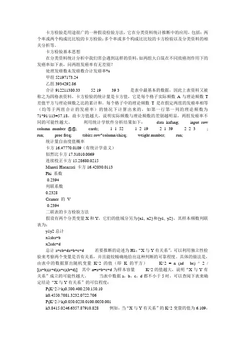
卡方检验是用途很广的一种假设检验方法,它在分类资料统计推断中的应用,包括:两个率或两个构成比比较的卡方检验;多个率或多个构成比比较的卡方检验以及分类资料的相关分析等。
卡方检验基本思想在分类资料统计分析中我们常会遇到这样的资料,如两组大白鼠在不同致癌剂作用下的发癌率如下表,问两组发癌率有无差别?处理发癌数未发癌数合计发癌率%甲组52197173.24乙组3934292.86合计912211380.33 52 19 39 3 是表中最基本的数据,因此上表资料又被称之为四格表资料。
卡方检验的统计量是卡方值,它是每个格子实际频数A与理论频数T 差值平方与理论频数之比的累计和。
每个格子中的理论频数T是在假定两组的发癌率相等(均等于两组合计的发癌率)的情况下计算出来的,如第一行第一列的理论频数为71*91/113=57.18,故卡方值越大,说明实际频数与理论频数的差别越明显,两组发癌率不同的可能性越大。
利用统计学软件分析结果如下:data kafang; input row column number @@; cards; 1 1 52 1 2 19 2 1 39 2 2 3 ; run; proc freq; tables row*column/chisq; weight number; run;统计量自由度值概率卡方16.47770.0109(有统计学意义)似然比卡方17.31010.0069连续校正卡方15.28680.0215Mantel-Haenszel 卡方16.42030.0113Phi 系数-0.2394列联系数0.2328Cramer 的V-0.2394二联表的卡方检验方法假设有两个分类变量X和Y,它们的值域分另为{x1, x2}和{y1, y2},其样本频数列联表为:y1y2总计x1aba+bx2cdc+d总计a+cb+da+b+c+d 若要推断的论述为H1:“X与Y有关系”,可以利用独立性检验来考察两个变量是否有关系,并且能较精确地给出这种判断的可靠程度。
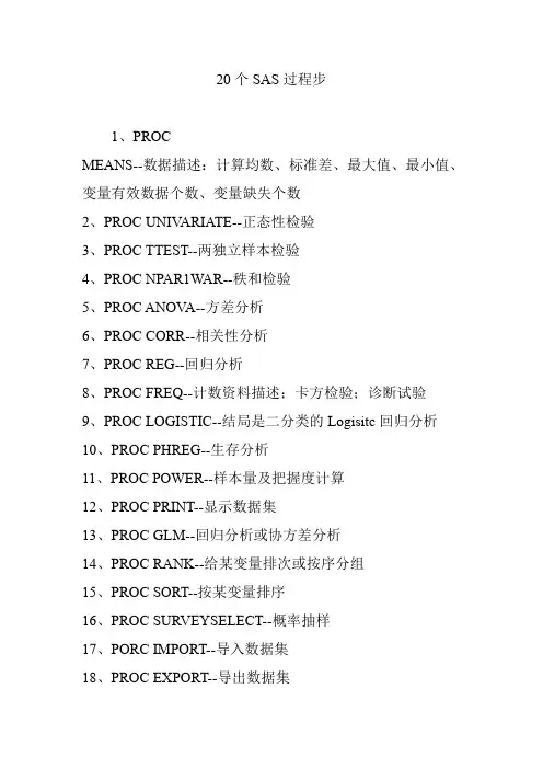
20个SAS过程步
1、PROC
MEANS--数据描述:计算均数、标准差、最大值、最小值、变量有效数据个数、变量缺失个数
2、PROC UNIV ARIATE--正态性检验
3、PROC TTEST--两独立样本检验
4、PROC NPAR1WAR--秩和检验
5、PROC ANOV A--方差分析
6、PROC CORR--相关性分析
7、PROC REG--回归分析
8、PROC FREQ--计数资料描述;卡方检验;诊断试验
9、PROC LOGISTIC--结局是二分类的Logisitc回归分析
10、PROC PHREG--生存分析
11、PROC POWER--样本量及把握度计算
12、PROC PRINT--显示数据集
13、PROC GLM--回归分析或协方差分析
14、PROC RANK--给某变量排次或按序分组
15、PROC SORT--按某变量排序
16、PROC SURVEYSELECT--概率抽样
17、PORC IMPORT--导入数据集
18、PROC EXPORT--导出数据集
19、PROC CONTENTS--产生一个数据集的头文件,包含了多种该数据集的信息
20、PROC TABULATE--输出报表。
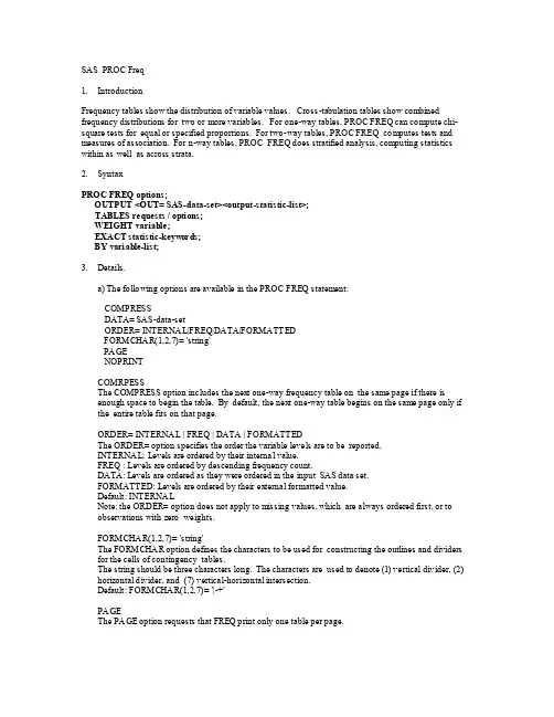
SAS PROC Freq1.IntroductionFrequency tables show the distribution of variable values. Cross-tabulation tables show combined frequency distributions for two or more variables. For one-way tables, PROC FREQ can compute chi-square tests for equal or specified proportions. For two-way tables, PROC FREQ computes tests and measures of association. For n-way tables, PROC FREQ does stratified analysis, computing statistics within as well as across strata.2.SyntaxPROC FREQ options;OUTPUT <OUT= SAS-data-set><output-statistic-list>;TABLES requests / options;WEIGHT variable;EXACT statistic-keywords;BY variable-list;3.Details.a) The following options are available in the PROC FREQ statement:COMPRESSDATA= SAS-data-setORDER= INTERNA L|FREQ|DATA|FORMATTEDFORMCHA R(1,2,7)= 'string'PA GENOPRINTCOMRPESSThe COMPRESS option includes the next one-way frequency table on the same page if there is enough space to begin the table. By default, the next one-way table begins on the same page only if the entire table fits on that page.ORDER= INTERNA L | FREQ | DATA | FORMATTEDThe ORDER= option specifies the order the variable levels are to be reported.INTERNA L: Levels are ordered by their interna l value.FREQ : Levels are ordered by descending frequency count.DATA: Levels are ordered as they were ordered in the input SAS data set.FORMATTED: Levels are ordered by their external formatted value.Default: INTERNA LNote: the ORDER= option does not apply to missing values, which are always ordered first, or to observations with zero weights.FORMCHA R(1,2,7)= 'string'The FORMCHA R option defines the characters to be used for constructing the outlines and dividers for the cells of contingency tables.The string should be three characters long. The characters are used to denote (1) vertical divider, (2) horizontal divider, and (7) vertical-horizontal intersection.Default: FORMCHA R(1,2,7)= '|-+'PA GEThe PA GE option requests that FREQ print only one table per page.NOPRINTThe NOPRINT option suppresses all printed output from PROC FREQ. Note that a NOPRINT options continues to be available in the TABLES statement. It suppresses printing of the tables, but allows printing of the statistics specified by the ALL, CHISQ, CMH, EXA CT, MEASURES, and PLCORR options.b) OUTPUT <OUT= SAS-data-set> <output-statistic-list>;The OUTPUT statement creates a SAS data set containing statistics computed by PROC FREQ. The output SAS data set can include any statistics requested in the TABLES statement. You can request these statistics by using keywords identical to the options used to request them in the TABLES statement: A GREE, A LL, CHISQ, CMH, CMH1, CMH2, EXA CT, MEASURES, and PLCORR. Or, request individual statistics by specifying one of the keywords listed below:AJCHI EXACT MCNEM PHI RSK11 SMDCRBDCHI JT MHCHI PLCORR RSK12 SMDRCCMHCOR KAPPA MHOR RDIF1 RSK21 STUTCCMHGA LAMCR MHRRC1 RDIF2 RSK22 TRENDCMHRMS LAMDAS MHRRC2 RRC1 RELRISK TSYMMCONTGY LAMRC N RRC2 RISKDIFF UCQ LGOR NMISS RROR RISKDIFF1 UCRCRAMV LGRRC1 PCHI RSK1 RISKDIFF2 URCEQKAPS LGRRC2 PCORR RSK2 SCORR WTKAPPAEQWTKAPS LRCHIOnly one OUTPUT statement is allowed for each execution of the FREQ procedure. Where there are multiple TABLES statements, the contents of the output SAS data set correspond to the last TABLES statement; when there are multiple table requests in a TABLES statement, the contents correspond to the last table request. For each stratum, there is one observation that contains the requested statistics. The names for the requested statistics are the names of the keywords enclosed in underscores. If a stati stic has a corresponding p-value, the name for the p-value is formed by adding P and an underscore before the keyword. Other variables included are BY variables, if any, and variables that identify the stratum.c) TABLES requests / options;The TABLES command requests tables be produced. Any number of TA BLES statements can be included. If no TA BLES statement is given, one-way frequencies for all of the variables in the data set are produced. To request a one-way frequency table for a variable, name the variable in a TABLES statement. For example: PROC FREQ;TA BLES a;For a crosstabulation table of two variables, give their names separated by an asterisk. The first variable's values form the rows of the table, and the second variable's values form the columns. For example: PROC FREQ; TABLES a*b;For n-way crosstabulation tables, the last variable's values form the columns; the next-to-last variable's values form the rows. Each level (or combination of levels) of the other variables form one stratum.A contingency table is produced for each stratum.TABLES requests / options ;Options that can be used in the TABLES statement:General LIST MISSING OUT= V5FMTRequest Statistical analysis:A GREE ALL CHISQ CL CMH CMH1CMH2 EXACT JT MEASURES PLCORR RELRISKRISKDIFF TESTF= TESTP= TRENDStatistical Details A LPHA= CONVERGE= MAXITER= SCORES=Request Additional Table informationCELLCHI2 CUMCOL DEVIATION EXPECTED MISSPRINT SPA RSE TOTPCT Suppress Printing NOCOL NOCUM NOFREQ NOPERCENT NOPRINT NOROWNOTE: see SAS online manual for more details.d) WEIGHT variable;Normally, each observation contributes a value of 1 to the frequency counts. When a WEIGHTstatement appears, each observation contributes the weighting variable's value for that observation.The values do not have to be integers. Negative values for the specified variable are allowed. Since negative values cannot correspond to actual frequencies, the total frequency, percentages, andstati stical calculations are undefined and, therefore, not printed when there are negative weights.If the value of the weight variable is missing or zero, the corresponding observation is ignored.Only one WEIGHT statement can be used, and that statement applies to counts collected for all tables.e) EXA CT statistic-keywords;The EXACT statement allows you to specify statistics for which to calculate exact p-values. You can request exact computations for groups of statistics by specifying keywords identical to the TABLES statement options AGREE, CHISQ, and MEASURES. You can request exact p-values for anindividual statistic by specifying the corresponding keyword in the following list. Note thatspecifying the keyword RROR requests exact confidence bounds for the odds ratio for 2x2 tables.JT MHCHI SCORR KAPPA PCHI TRENDLRCHI PCORR WTKAP MCNEM RRORf) BY <DESCENDING> variables ... <NOTSORTED>;A BY statement is used with a procedure to obtain separate analyses on observations in groupsdefined by the BY variables. The data set being processed need not have been previously sorted by the SORT procedure. However, the data set must be in the same order as though PROC SORT had sorted it unless NOTSORTED is specified. If you have used a FORMAT or ATTRIB statement to group a continuous variable into discrete groups, the BY statement creates BY groups based on the formatted values. You can also ensure that variables are processed in ascending order by creating an index for one or more variables in the SAS data set. The usages of the BY statement differ in each procedure. Please refer to the Users' Guide for the details.。

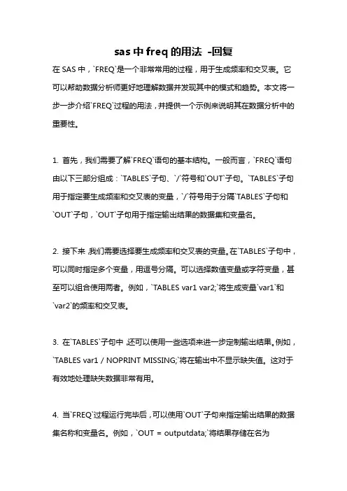
sas中freq的用法-回复在SAS中,`FREQ`是一个非常常用的过程,用于生成频率和交叉表。
它可以帮助数据分析师更好地理解数据并发现其中的模式和趋势。
本文将一步一步介绍`FREQ`过程的用法,并提供一个示例来说明其在数据分析中的重要性。
1. 首先,我们需要了解`FREQ`语句的基本结构。
一般而言,`FREQ`语句由以下三部分组成:`TABLES`子句、`/`符号和`OUT`子句。
`TABLES`子句用于指定要生成频率和交叉表的变量,`/`符号用于分隔`TABLES`子句和`OUT`子句,`OUT`子句用于指定输出结果的数据集和变量名。
2. 接下来,我们需要选择要生成频率和交叉表的变量。
在`TABLES`子句中,可以同时指定多个变量,用逗号分隔。
可以选择数值变量或字符变量,甚至可以组合使用两者。
例如,`TABLES var1 var2;`将生成变量`var1`和`var2`的频率和交叉表。
3. 在`TABLES`子句中,还可以使用一些选项来进一步定制输出结果。
例如,`TABLES var1 / NOPRINT MISSING;`将在输出中不显示缺失值。
这对于有效地处理缺失数据非常有用。
4. 当`FREQ`过程运行完毕后,可以使用`OUT`子句来指定输出结果的数据集名称和变量名。
例如,`OUT = outputdata;`将结果存储在名为`outputdata`的数据集中。
这样,我们可以在进一步分析时使用这些结果。
5. 另外,`FREQ`过程还可以生成卡方检验、精确检验和倾向分数。
这些统计指标可以帮助我们判断样本数据是否符合理论分布,并进行统计推断。
现在,让我们通过一个具体的示例来进一步说明`FREQ`过程的用法。
假设我们有一个数据集包含了学生的性别(gender)和考试成绩(score)两个变量。
我们希望通过`FREQ`过程来分析性别和考试成绩之间的关系。
首先,我们需要指定要生成频率和交叉表的变量。
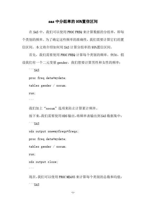
sas中分组率的95%置信区间在SAS中,我们可以使用PROC FREQ来计算数据的分组率,即每个类别的频率。
为了确定这些频率的准确性,我们需要计算它们的置信区间。
本文将介绍如何用SAS计算分组率的95%置信区间。
首先,我们需要使用PROC FREQ计算每个类别的频率。
例如,假设我们有一个二元变量gender,我们想要计算男性和女性的频率: ```SASproc freq data=mydata;tables gender / nocum;run;```我们加上“nocum”选项来防止计算累计频率。
接下来,我们需要使用ODS输出,将频率表输出到SAS数据集中: ```SASods output onewayfreqs=freqs;proc freq data=mydata;tables gender / nocum;run;ods output close;```现在,我们可以使用PROC MEANS来计算每个类别的总数和均值: ```SASproc means data=freqs sum mean;var count;output out=summary sum=total n=n;run;```我们使用“sum”选项计算总数,使用“n”选项计算每个类别的观测数。
最后,我们可以使用PROC IML来计算95%置信区间:```SASproc iml;use summary;read all var {'total' 'n'} into X;close summary;alpha = 0.05;crit = quantile('t', 1-alpha/2, n-1);stderr = sqrt(X[,1]*(1-X[,1])/X[,2]);ci = X[,1] + crit*stderr;print ci[colname={'Lower' 'Upper'}],format=8.6;quit;```我们使用PROC IML来读入我们之前计算的总数和观测数,然后计算95%置信区间。

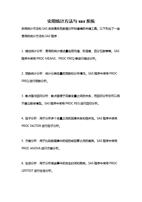
实用统计方法与sas系统
实用统计方法和SAS系统是实现数据分析和建模的关键工具。
以下列出了一些常用的统计方法和SAS程序:
1. 描述统计分析:常用的统计描述量包括均值、标准差、百分位数等等。
SAS 程序中使用PROC MEANS、PROC FREQ等进行描述分析。
2. 频数统计分析:统计分类变量的频数和分布情况。
SAS程序中使用PROC FREQ进行频数分析。
3. 散点图与回归分析:散点图便于观察变量之间的关系,而回归分析则可以用于建立数学模型。
SAS程序中使用PROC REG进行回归分析。
4. 因子分析:用于分析多个变量之间的因果关系和相关性。
SAS程序中使用PROC FACTOR进行因子分析。
5. 方差分析:用于比较数据集中的组别或因素之间的差异。
SAS程序中使用PROC ANOVA进行方差分析。
6. 生存分析:用于分析某些事件的发生时间和概率。
SAS程序中使用PROC LIFETEST进行生存分析。
7. 分类树(决策树):用于建立分类模型。
SAS程序中使用PROC ARBOR进行分类树分析。
总之,通过适当使用SAS程序和搭配合适的统计方法,可以更加准确地进行数据分析和模型建立。
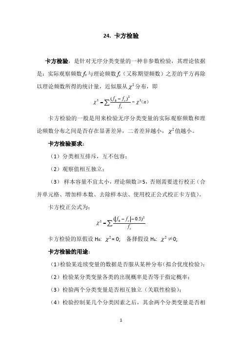
24. 卡方检验卡方检验,是针对无序分类变量的一种非参数检验,其理论依据是:实际观察频数f 0与理论频数f e (又称期望频数)之差的平方再除以理论频数所得的统计量,近似服从2χ分布,即)(n f f f ee 2202~)(χχ∑-= 卡方检验的一般是用来检验无序分类变量的实际观察频数和理论频数分布之间是否存在显著差异,二者差异越小,2χ值越小。
卡方检验要求:(1)分类相互排斥,互不包容; (2)观察值相互独立;(3) 样本容量不宜太小,理论频数≥5,否则需要进行校正(合并单元格、增加样本数、去除样本法、使用校正公式校正卡方值)。
卡方校正公式为:∑--=ee f f f 202)5.0(χ卡方检验的原假设H 0: 2χ= 0; 备择假设H 1: 2χ≠0; 卡方检验的用途:(1)检验某连续变量的数据是否服从某种分布(拟合优度检验); (2)检验某分类变量各类的出现概率是否等于指定概率; (3)检验两个分类变量是否相互独立(关联性检验); (4)检验控制某几个分类因素之后,其余两个分类变量是否相互独立;(5)检验两种方法的结果是否一致,例如两种方法对同一批人进行诊断,其结果是否一致。
(一)检验单样本某水平概率是否等于某指定概率一、单样本案例例如,检验彩票中奖号码的分布是否服从均匀分布(概率=某常值);检验某产品市场份额是否比以前更大;检验某疾病的发病率是否比以前降低。
有数据文件:检验“性别”的男女比例是否相同(各占1/2)。
1. 【分析】——【非参数检验】——【单样本】,打开“单样本非参数检验”窗口,【目标】界面勾选“自动比较观察数据和假设数据”2.【字段】界面,勾选“使用定制字段分配”,将变量“性别”选入【检验字段】框;注意:变量“性别”的度量标准必须改为“名义”类型。
3. 【设置】界面,选择“自定义检验”,勾选“比较观察可能性和假设可能性(卡方检验)”;4. 点【选项】,打开“卡方检验选项”子窗口,本例要检验男女概率都=0.5,勾选“所有类别概率相等”;注:若有类别概率不等,需要勾选“自定义期望概率”,在其表中设置各类别水平及相应概率。
sas课后习题答案SAS课后习题答案SAS(Statistical Analysis System)是一种广泛应用于数据分析和统计建模的软件工具。
它提供了丰富的功能和强大的数据处理能力,被广泛应用于各个领域的数据分析工作中。
在学习SAS的过程中,课后习题是一种非常重要的练习方式,可以帮助学生巩固所学的知识并提高实际应用能力。
本文将为大家提供一些常见SAS课后习题的答案,希望能对大家的学习有所帮助。
一、基础习题答案1. 请编写SAS代码,计算一个数据集中某个变量的平均值。
解答:```data dataset;input variable;datalines;1234;run;proc means data=dataset mean;var variable;```以上代码中,我们首先创建了一个名为dataset的数据集,并输入了一个名为variable的变量。
然后使用proc means过程计算了变量variable的平均值。
2. 请编写SAS代码,将两个数据集按照某个变量进行合并。
解答:```data dataset1;input id variable1;datalines;1 102 203 30;run;data dataset2;input id variable2;datalines;1 1002 2003 300;data merged_dataset;merge dataset1 dataset2;by id;run;```以上代码中,我们首先创建了两个数据集dataset1和dataset2,并分别输入了id和variable1,以及id和variable2两个变量。
然后使用merge语句将两个数据集按照id变量进行合并,生成了一个名为merged_dataset的新数据集。
二、进阶习题答案1. 请编写SAS代码,对一个数据集进行排序,并输出排序后的结果。
解答:```data dataset;input variable;datalines;3142;run;proc sort data=dataset out=sorted_dataset;by variable;run;```以上代码中,我们首先创建了一个名为dataset的数据集,并输入了一个名为variable的变量。
20. 用PROC FREQ计算频数及卡方检验
(一)卡方检验
一、卡方分布
k 个相互独立的标准正态分布变量的平方和服从自由度为k 的卡方分布。
二、卡方检验概述
卡方检验,由英国统计学家Karl Pearson得到,主要应用于计数数据(定性变量中的无序分类变量)的分析,对于总体的分布不作任何假设,因此它属于非参数检验法。
理论证明,实际观察频数(f0)与理论频数(f e, 又称期望频数)之差的平方再除以理论频数所得的统计量,近似服从卡方分布,可表示为:
)(n f f f e e 22
02
~)(χχ∑-= 这是卡方检验的原始公式,其中当f e 越大,近似效果越好。
显然f o 与f e 相差越大,卡方值就越大;f o 与f e 相差越小,卡方值就越小;因此它能够用来表示f o 与f e 相差的程度。
根据这个公式,卡方检验的一般问题是要检验名义型变量的实际观测频数和理论频数分布之间是否存在显著差异。
一般卡方检验要求:① 分类相互排斥,互不包容;② 观察值相互独立;③ 样本容量不宜太小,理论频数≥5,否则需要进行校正。
如果个别单元格的理论频数小于5,处理方法有四种:
(1)单元格合并法;
(2)增加样本数;
(3)去除样本法;
(4)使用校正公式。
当期望次数小于5时,应该用校正公式计算卡方值:
∑--=e e f f f 2
02)5.0(χ
二、卡方检验的原理
1. 卡方检验所检测的是样本观察频数与理论(或总体)频数的差异性;
2. 理论或总体的分布状况,可用统计的期望值(理论值)来体现;
3. 卡方的统计原理,是取观察频数与期望频数相比较。
当观察频数与期望频数完全一致时,2χ值为0;观察频数与期望频数越接近,两者之间的差异越小,2χ值越小;观察频数与期望频数差别越大,两者之间的差异越大,2χ值越大。
一旦2χ值大于某一个临界值,即可获得显著的统计结论。
4. 步骤:
原假设H0: 2χ= 0; 备择假设H1: 2χ≠0;
根据数据计算卡方值、P值(右尾面积);
若P值≤α,则拒绝H0; 若P值>α,则接受H0.
三、卡方检验的应用
1. 拟合优度检验
检验单个多项分类名义型变量的各分类间的实际观测次数(根据样本数据得到的实计数)与理论次数(根据理论或经验得到的期望次数)之间是否一致、或者服从理论上的某种分布?这一类检验称为拟合性检验。
其自由度通常为分类数减去1。
2. 各变量间的独立性检验(定性变量列联表)
两个或两个以上因素多项分类的计数资料分析,也就是研究两类变量之间的关联性和依存性问题。
如果两变量无关联即相互独立,说明对于其中一个变量而言,另一变量多项分类次数上的变化是在无差
范围之内;如果两变量有关联即不独立,说明二者之间有交互作用存在。
独立性检验一般采用列联表的形式记录观察数据, 列联表是由两个以上的变量进行交叉分类的频数分布表,是用于提供基本调查结果的最常用形式,可以清楚地表示定类变量之间是否相互关联。
其自由度是:(行数-1)×(列数-1)
(二)PROC FREQ过程步
一、基本语法:
PROC FREQ data = 数据集;
TABLES 行变量* 列变量/ options;
<WEIGHT 权重变量>;
说明:结果将以表格形式(频数表)输出,
TABLES a—单向频数表;
TABLES a*b—a为行,b为列的双向频数表;
TABLES a*b*c—a为分层,b为行,c为列的三维频数表;
TABLES a*(b c)—等价于“TABLES a*b a*c”;
可选项:
(1)AGREE
做配对卡方检验;
(2)CHISQ
做独立性和关联度的卡方检验;
(3)CL
输出关联度的置信限;
(4)CMH
输出Cochran-Mantel-Haenszel统计量,特别对分层二维表;
(5)EXACT
做Fisher精确检验;
(6)MEASURES
输出Pearson and Spearman相关系数、gamma、
Kendall's tau-b、Stuart's tau-c、Somer's D、lambda、
odds ratios、risk ratios、置信区间的关联度;
(7)RELRISK
输出2×2表的相对风险度;
(8)TREND
对趋势做Cochran-Armitage检验;
(9)NOROW, NOCOL, NOPERCENT
不输出行百分比、列百分比、百分比;
二、绘制PROC FREQ的图表
默认也会输出PROC FREQ的图表,若要输出指定图表,需要在TABLES语句中,使用绘图可选项“PLOTS = (plot-list);”即可。
可以绘制频数图、优势比图、Agreement图、偏差图、以及两类带Kappa 统计量和置信限的图。
基本语法:
PROC FREQ data = 数据集;
TABLES variable1 * variable2 / options PLOTS = (plot-list);
可选绘图类型:
AGREEPLOT——双向(配对)表
CUMFREQPLOT——单向表
DEVIATIONPLOT——单向(卡方检验)表
FREQPLOT——(任意)
KAPPAPLOT——三维表
ODDSRATIOPLOT——h×2×2(MEASURES or RELRISK)
RELREISKPLOT——h×2×2(MEASURES or RELRISK)
RISKDIFFPLOT——h×2×2(RELRISK)
WTKAPPAPLOT——h×r×r (r>2) (配对表)
注:FREQPLOT可以加选项,例如分组条形图默认是竖直排列,若要改用水平排列,可以用:
TABLES variable1 * variable2 / PLOTS = FREQPLOT(TWOWAY = GROUPHORIZONTAL);
若要堆叠分组条形,用“TWOW AY=STACKED”。
例1一组常规公交车(R: Regular)和快速公交车(E: Express)的延误(L: Late)或准时(O: On Time)的数据(C:\MyRawData\Bus.dat):
读入数据,用PROC FREQ过程步计算频数,并做卡方检验。
代码:
infile'c:\MyRawData\Bus.dat';
input BusType $ OnTimeOrLate $ @@;
run;
proc format;
value $type 'R'='Regular'
'E'='Express';
value $late 'O'='On Time'
'L'='Late';
run;
proc freq data = bus;
tables BusType * OnTimeOrLate / NOROW NOCOL CHISQ PLOTS=FREQPLOT(TWOWAY=GROUPHORIZONTAL);
format BusType $Type. OnTimeOrLate $Late.;
运行结果:
程序说明:
(1)常规公交车延迟率为61.9%, 快速公交车延迟率为24.14%;
(2)卡方检验的卡方值为7.2386,P值为0.0071<α=0.05; 说明两种公交车的延迟率有着明显差异,结果具有统计学意义;同时也说明“延误或准时与否”与选择哪种公交车是有关系的;另外,Fisher 精确检验的结果也支持这一结论。