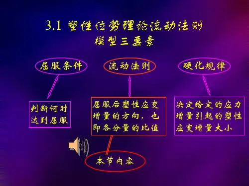
弹塑性力学第三章
- 格式:ppt
- 大小:286.00 KB
- 文档页数:35

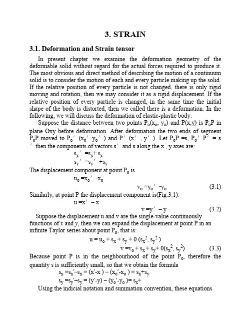
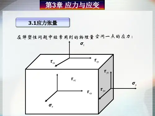
3. STRAIN3.1. Deformation and Strain tensorIn present chapter we examine the deformation geometry of the deformable solid without regard for the actual forces required to produce it. The most obvious and direct method of describing the motion of a continuum solid is to consider the motion of each and every particle making up the solid. If the relative position of every particle is not changed, there is only rigid moving and rotation, then we may consider it as a rigid displacement. If the relative position of every particle is changed, in the same time the initial shape of the body is distorted, then we called there is a deformation. In the following, we will discuss the deformation of elastic-plastic body.Suppose the distance between two points P o(x o, y o) and P(x,y) is P o P in plane Oxy before deformation. After deformation the two ends of segment P o P moved to P o′(x o′y o′) and P′(x′, y′). Let P o P =s, P o′P′= s ′then the components of vectors s′and s along the x , y axes are:s x′=s x+ s xs y′=s y′+s yThe displacement component at point P o isu o =x o′‑x ov o =y o′‑y o (3.1) Similarly, at point P the displacement component is(Fig.3.1):u =x′– xv =y′– y (3.2) Suppose the displacement u and v are the single-value continuously functions of x and y, then we can expand the displacement at point P in an infinite Taylor series about point P o, that is:u = u o + s x + s y + 0 (s x2, s y2 )v =v o + s x + s y+ 0(s x2, s y2) (3.3) Because point P is in the neighbourhood of the point P o, therefore the quantity s is sufficiently small, so that we obtain the formulas x =s x′–s x = (x′-x ) – (x o′-x o ) = s x+s ys y =s y′–s y = (y′-y) – (y o′-y o )= s x+Using the indicial notation and summation convention, these equationsmay be written more compactly ass i = u i ,j s j (3.4) where (i,j =x, y ) in two dimensional case, ( i,j =x, y, z ) in three dimensional case, this givesu i , j = (3.5) which is so called relative displacement tensor.Fig. 3.1 displacement of a segmentIn order to get a clear idea of strain, we shall return by considering the figure 3.1,from which we know there is a rigid displacement only, when the segment s moved to s′, without any deformation. The length of s is not changed, then we obtains2 =s′ 2 = ( s x + s x)2 +( s y + s y)2 (3.6)Expanding above formula (3.6) and neglecting the high-order small quantity s i , we obtains2= s2 + 2 (s x s x + s y s y )From which we haves x s x + s y s y= 0ors i s i = 0 (3.7) From equation (3.4) we obtaineds i u i , j s j = 0 (3.8) ors x2 +s x s y + s y2 = 0In view of the arbitrary of s x , s y , we have(3.9) Similar to above discussion for planes Oyz and Oxz we can obtain another three conditions:= 0+ = = 0Therefore we haveu i , j = --u j ,i (3.10) It means that the relative displacement tensor of rigid-body motion must be a skew-symmetric tensorEvery second-order tensor can be decomposed into two parts uniquely, one is a symmetric tensor and another is a skew-symmetric. Hence we can write u i ,j as the following form:u i , j = ( u i , j + u j , i ) + ( u i , j – u j , i ) ( 3.11) oru i , j =i j + i j (3.11a) where= (3.12)ij= (3.13)ijand ij are the strain tensor and rotation tensor respectively for two-ijdimensional case.From equation (3.11) we can easy write the expression of strain tensor and rotation tensor for three-dimensional cases.In this case, equation (3.4) may be written ass i = ij s j (3.14) If segment s is parallel x-axis, then we haves x = s, s y = 0and= x = = (3.15)xxIt is clear that x is the unit elongation ( compression) of a unit line element vector paralleled x-axis, and the same to y , z , so called line strain or normal strain.If vector s1and vector s2are parallel axes O x, O y respectively before deformation,i, j are the unit vector along the direction of O x, O y axes, respectively. ( Fig. 3.2 ) Therefore we haves1 = i s1 s2 = i s2After deformation s1, s2became to s1’, s2’ , respectively. Then we haves1′ = i (s1x + s1) + j s1ys2′ = i s2x+j (s2y +s2 )Fig.3.2 The change of angle between two vectorsLet the angle between vectors s1’and s2’, then from the definition of inner product of two vectors, we obtains1′s2′= s1′ s2′ cos (3.16) and s1′s2′= (s1x′ i+s1y′ j) (s2x′ i+s2y′ j )=s1x′ s2x′ +s1y′ s2y′where s1y′ =s1y s2x′ = s2xNeglecting the two-order small quantity of s, we haves1′s2′ = s1s2x + s2s1y (3.17)Substituting this relation into the expression (3.16) and neglecting high-order small quantity again, after some reduction that we can obtaincos(s1s2x+s2s1y) / s1s2 =+Let the change in the angle between line elements s1, s2 , after deformation is, considering that is a small quantity too, then we havecos= cos (/2—) =sin=From xy = yx , we find=xy + yx= 2xySo that the strain component xy is seen to represent simply one- half the change in the angle between line elements lying initially in the x and y axes directions. A similar interpretation also applies to the strain components xz and yz, that isLet the angle between the two lines which is perpendicularly each other and coincident with positive direction of axes O x, O y before deformation have been changed after deformation, if the changed quantity is xy namely shear strain, then= = 2xy = + (3.19)xyor (3.19’ )In the following, we customarily take positive sign (or negative sign ) of shear strain, when the perpendicular angle between two coordinate axes is decreased ( or negative sign ). The strain components are clearly in two-dimensional case are= , y =, xy= + (3.20)xand in three-dimensional case are (in compact form )=u i , i ( i , j= x,y,z ) (3.21)ii= u i, j+u j , i (3.21′)ijwhere u x u, u y v, u z w, and as before by using the von. Karman’s notation:, yyy , zz=z , andxxx= ji (3.22)ijEquation (3.21) is the strain displacement relation:=1/2 ( u i ,j + u j , i ) (i ,j =x,y,z ) (3.23)ijIt is clearly when i =j ,we get a normal strain , ij , we get a shear strain. In addition we have= ji (3.24)ij3.2. Principal Strain and Octahedral StrainIn last chapter, it has been demonstrated that there exist at least three mutually orthogonal planes, which have no shear stress acting on them, that is, the principal planes and their associated principal directions, known as principal axes. In the analysis of strain at a point, such principal axes also exist. As we known, that the principal axis or direction is the direction for which the shear strains would be zero. The corresponding strains are called principal strains. Obviously, the direction of principal strain is coincides with principal direction. This strain is the normal strain. Other word, if the outward normal of a plane is coincides with the principal direction, then this plane is just the principal plane.Suppose vectors s n, coincide with the outward normal line of plane ABC ( Fig. 3.3 ).In the process of deformation the direction of s n is unchanged and only changed its length. If the quantity of changing is s n , then we haves n / s n =s x / s x = s y / s y = s z / s zWhere s x , s y , s z and s x , s y , z are the projection of s n , and s n on axes Ox, Oy, Oz respectively. Considering thatFig. 3.3 Principal strainn(3.25)Then we haves n = n s n (3.26) As we have discussed before, the relative displacement vector corresponding to pure deformation is called the strain vector, then we obtain from equation (3.14)s i= ij s j (3.27) From equations (2.5) and (2.6) we have(ij –ijn ) s j = 0 (3.28) Similarly, we have a cubic algebra equation of n:n 3 – I1′n2 +I2′n – I3′ = 0 (3.29)whereI1′ =I2′ = xy +yz +zx – (xy2 +yz2 +zx2 ) (3.30)I3′==xyz+2xyyzzx –(xyz2+yzx2+zyx2)Where I1′ I2′ and I3′are called the first, second, and third invariant of strain tensor. In terms of the principal strain 1, 2, and3, we haveI1′ =1+2+ 3I2′ =12+23+31 (3.31)I3′ = 123The shear strain for some directions at a point that assume stationary values are called the principal shear strains. The principal shear strain and the corresponding directions can therefore be obtained in exactly the same manner as for stresses. Thus, designating the maximum shear strain by 1, 2, and 3 , we can write1= (2 - 3)2= (1 - 3) (3.32)3= (1 - 2)The octahedral shear strain is= [(x –y)2 +(y –z)2 +(z –x)2 +6(xy2 +yz2 +zx2 )]1/2 (3.33)8or= (I1′ 2 – 3I2′ )1/2 (3.34)83.3. Strain Deviator TensorIn the same manner as for stresses we can obtain the strain deviator tensor and their invariant . As in the case of the stress tensor, the strain tensor can be decomposed into two parts too, a spherical part associated with a change in volume, and a deviatoric part associated with a change in shape distortion. that is ,= e ij +kk ij (3.35)ijwhere e ij is defined here as the strain deviator tensor and 1/3(kk ) is the mean strain or the hydrostatic strain. Thus, the strain deviator tensor e ij becomes(3.36)The invariants of the strain deviator tensor e ij are analogous to those obtained for stress deviator tensor s ij, these deviatoric strain invariants appear in the cubic equation of the determinant equation [e ij- e ij]=0.e3- J1′e2 – J2′e – J3′ = 0 (3.37)whereJ1′ =e ii =0J2′ =e1e2+e2e3+e3e1 (3.38)J3′= e1e2e3orJ1′ = 0J2′ = 1/3 (I1′ – 3I2′ )J3′= 1/27 (2I1′ 3 – 9I1′I2′ +27I3′ ) (3.39) It can be seen that the octahedral shear strain 8is related to the second invariant of the deviator strain tensor J’2, as was the case for stresses:(3.40)Now we introduce two special quantities, which is useful in theory of plasticity, the effective strain(3.41) and shear strain strength (or equivalent shear strain )(3.42) 3.4. Equations of Strain CompatibilityFor static elasticity in the last chapter, it has been pointed out that we must establish the equilibrium equations to ensure that the body is always in a equilibrium state. In the analysis of strain , however, there must be some conditions to be imposed on the strain components so that the deformed body remains continuous. In mathematical review, that the displacement function u, v, and w must be the continuum single-value function in their definite region. After deformation, there are no cracks, no rips, and no folds in whole body. The mathematical restriction on strain components which ensure that this is the case are known as the compatibility equations.To establish these equations, let us first suppose that displacement components do indeed exist. In this case, we have that the strain components2ij = u i,j + u j,I (3.44) It can be shown that the compatibility equations for a simply connected region may be written in the form+ kl , ji – ik , jl – jl ,ik = 0 (3.45)ij , klIn other hand, if we take the second derivative of x with respect to y, and y with respect to x, then after added together we can obtained(3.46) Equation (3.46) is the compatibility equation for two-dimensional problem.Expanding equation (3.45), we get(3.47)These 6 compatibility equations are the necessary and sufficient conditions required to ensure that the strain components give single-valued continuous displacements for a simply connected region. It is clear that the compatibility equations are introduced from the equations of strain-displacement relation. Therefore, if we can find the displacement functions u, v, w and strain components correctly according to strain-displacement relations, then the strain compatibility equations will be satisfied spontaneously.Problems1. Expand , that is write it in conventional notation.2. Given the strain tensorFind : (a) principal strains; (b) principal directions; (c) octahedral shear strain; (d) invariance of strain.Anwser: (a) -2.764 -7.236; (b) inclined to x-axis; (c) (d)3. Prove I1′is a invariant while coordinate system is rot。