温度模拟
- 格式:pdf
- 大小:355.32 KB
- 文档页数:6

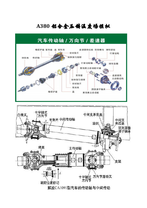
A380铝合金压铸温度场模拟如图所示汽车传动轴,用A380铝合金半固态触变压铸成型工艺可获得重量轻、强度高、综合力学性能优越的零件,能够满足未来汽车工业轻量化、节能环保的要求。
查相关资料,A380铝合金半固态触变压铸成型工艺的浆料温度为570℃,模具预热温度为200℃,冷却水对流换热系数为450W/(m2·℃), A380铝合金密度为2730㎏/m3, 模具材料密度为7800㎏/m3,导热系数为21W/(m·℃),比热为110J/(㎏·℃)。
A380铝合金热性能参数相关尺寸在建模时提及,不赘述。
为简化建模,只取冷却水包络面以内的模具和铸件建模。
操作步骤1.定义工作标题和文件名(1)指定工作文件名:执行Utinity Menu/File/Change Jobname命令,在【Enter new Name】文本框中输入“WBA.file”,单击OK按钮。
(2)指定工作标题:执行Utinity Menu/File/Change Title命令,输入“Casting Solidification”, 单击OK按钮。
2.定义单元类型和材料属性(1)定义单元类型:执行Main Menu/Preprocessor/Element Type/Add、Edit、Delete命令,单击Add按钮,选择如下图选项,单击OK按钮。
(2)定义材料特性:执行Main Menu/Preprocessor/Material Props/ Material Models命令,双击【Material Models Available】列表框中的“Thermal/Conductivity/Isotropic”选项,定义模具导热系数(KXX)为“21”,接着双击“Thermal/Specific heat”选项, 定义模具比热(C)为“110”,单击OK按钮。
接着双击“Thermal/Density”选项, 定义模具密度(DENS)为“7800”,单击OK按钮。

传热大作业二维导热物体温度场的数值模拟(等温边界条件)姓名:班级:学号:墙角稳态导热数值模拟(等温条件)一、物理问题有一个用砖砌成的长方形截面的冷空气空道,其截面尺寸如下图所示,假设在垂直于纸面方向上冷空气及砖墙的温度变化很小,可以近似地予以忽略。
在下列两种情况下试计算:(1)砖墙横截面上的温度分布;(2)垂直于纸面方向的每米长度上通过砖墙的导热量。
外矩形长为3.0m ,宽为2.2m ;内矩形长为2.0m ,宽为1.2m 。
第一种情况:内外壁分别均匀地维持在0℃及30℃;第二种情况:内外表面均为第三类边界条件,且已知:外壁:30℃ ,h1=10W/m2·℃,内壁:10℃ ,h2= 4 W/m2·℃砖墙的导热系数λ=0.53 W/m ·℃由于对称性,仅研究1/4部分即可。
二、数学描写对于二维稳态导热问题,描写物体温度分布的微分方程为拉普拉斯方程 02222=∂∂+∂∂y t x t这是描写实验情景的控制方程。
三、方程离散用一系列与坐标轴平行的网格线把求解区域划分成许多子区域,以网格线的交点作为确定温度值的空间位置,即节点。
每一个节点都可以看成是以它为中心的一个小区域的代表。
由于对称性,仅研究1/4部分即可。
依照实验时得点划分网格:建立节点物理量的代数方程对于内部节点,由∆x=∆y ,有 )(411,1,,1,1,-+-++++=n m n m n m n m n m t t t t t由于本实验为恒壁温,不涉及对流,故内角点,边界点代数方程与该式相同。
设立迭代初场,求解代数方程组。
图中,除边界上各节点温度为已知且不变外,其余各节点均需建立类似3中的离散方程,构成一个封闭的代数方程组。
以C t 000=为场的初始温度,代入方程组迭代,直至相邻两次内外传热值之差小于0.01,认为已达到迭代收敛。
四、编程及结果1) 源程序#include <stdio.h>#include <math.h>int main(){int k=0,n=0;double t[16][12]={0},s[16][12]={0}; double epsilon=0.001;double lambda=0.53,error=0; double daore_in=0,daore_out=0,daore=0; FILE *fp;fp=fopen("data3","w");for(int i=0;i<=15;i++)for(int j=0;j<=11;j++){if((i==0) || (j==0)) s[i][j]=30;if(i==5)if(j>=5 && j<=11) s[i][j]=0;if(j==5)if(i>=5 && i<=15) s[i][j]=0;}for(int i=0;i<=15;i++)for(int j=0;j<=11;j++)t[i][j]=s[i][j];n=1;while(n>0){n=0;for(int j=1;j<=4;j++)t[15][j]=0.25*(2*t[14][j]+t[15][j-1]+t[15][j+1]);for(int i=1;i<=4;i++)t[i][11]=0.25*(2*t[i][10]+t[i-1][11]+t[i+1][11]);for(int i=1;i<=14;i++)for(int j=1;j<=4;j++)t[i][j]=0.25*(t[i+1][j]+t[i-1][j]+t[i][j+1]+t[i][j-1]);for(int i=1;i<=4;i++)for(int j=5;j<=10;j++)t[i][j]=0.25*(t[i+1][j]+t[i-1][j]+t[i][j+1]+t[i][j-1]);for(int i=0;i<=15;i++)for(int j=0;j<=11;j++)if(fabs(t[i][j]-s[i][j])>epsilon)n++;for(int i=0;i<=15;i++)for(int j=0;j<=11;j++)s[i][j]=t[i][j];k++;//printf("%d\n",k);}for(int j=0;j<=5;j++){ for(int i=0;i<=15;i++){ printf("%4.1f ",t[i][j]);fprintf(fp,"%4.1f ",t[i][j]);}printf("\n");fprintf(fp,"\n");}for(int j=6;j<=11;j++){ for(int i=0;i<=5;i++){ printf("%4.1f ",t[i][j]);fprintf(fp,"%4.1f ",t[i][j]);}fprintf(fp,"\n");printf("\n");}for(int i=1;i<=14;i++)daore_out+=(30-t[i][1]);for(int j=1;j<=10;j++)daore_out+=(30-t[1][j]);daore_out=4*(lambda*(daore_out+0.5*(30-t[1][11])+0.5*(30-t[15][1])));for(int i=5;i<=14;i++)daore_in+=t[i][4];for(int j=5;j<=10;j++)daore_in+=t[4][j];daore_in=4*(lambda*(daore_in+0.5*t[4][11]+0.5*t[15][4]));error=abs(daore_out-daore_in)/(0.5*(daore_in+daore_out));daore=(daore_in+daore_out)*0.5;printf("k=%d\n内墙导热=%f\n外墙导热=%f\n平均值=%f\n偏差=%f\n",k,daore_in,daore_out,daore,error);}2)结果截图七.总结与讨论1.由实验结果可知:等温边界下,数值解法计算结果与“二维导热物体温度场的电模拟实验“结果相似,虽然存在一定的偏差,但由于点模拟实验存在误差,而且数值解法也不可能得出温度真实值,同样存在偏差,但这并不是说数值解法没有可行性,相反,由于计算结果与电模拟实验结果极为相似,恰恰说明数值解法分析问题的可行性。

前言可编程控制器是一种应用很广泛的自动控制装置,它将传统的继电器控制技术、计算机技术和通讯技术融为一体,具有控制能力强、操作灵活方便、可靠性高、适宜长期连续工作的特点,非常适合温度控制的要求。
在工业领域,随着自动化程度的迅速提高,用户对控制系统的过程监控要求越来越高,人机界面的出现正好满足了用户这一需求。
人机界面可以对控制系统进行全面监控,包括过程监测、报警提示、数据记录等功能,从而使控制系统变得操作人性化、过程可视化,在自动控制领域的作用日益显著。
本文主要介绍了基于三菱公司FX2N系列的可编程控制器和亚控公司的组态软件组态王的某一对象温度控制系统的设计方案。
编程时调用了编程软件STEP 7 -Micro WIN中自带的PID控制模块,使得程序更为简洁,运行速度更为理想。
利用组态软件组态王设计人机界面,实现控制系统的实时监控、数据的实时采样与处理。
目录第一章概述 (2)第二章总方案 (3)2.1 系统框图 (3)2.2 下位机设计 (4)2.2.1 元件选择 (6)2.3 上位机设计 (8)2.3.1 监控主界面 (9)2.3.2 实时趋势曲线 (10)2.3.3 历史趋势曲线 (11)2.3.4 报警窗口 (11)2.3.5 设定画面 (12)2.3.6 变量设置 (13)2.3.7 动画连接 (15)第三章总结 (17)第四章参考文献 (17)1第一章概述温度控制在电子、冶金、机械等工业领域应用非常广泛。
由于其具有工况复杂、参数多变、运行惯性大、控制滞后等特点,它对控制调节器要求极高。
目前,仍有相当部分工业企业在用窑、炉等烘干生产线,存在着控制精度不高、炉内温度均匀性差等问题,达不到工艺要求,造成装备运行成本费用高,产出品品质低下,严重影响企业经济效益,急需技术改造。
近年来,国内外对温度控制器的研究进行了广泛、深入的研究,特别是随着计算机技术的发展,温度控制器的研究取得了巨大的发展,形成了一批商品化的温度调节器,如:职能化PID、模糊控制、自适应控制等,其性能、控制效果好,可广泛应用于温度控制系统及企业相关设备的技术改造服务。

传热大作业二维导热物体温度场的数值模拟(等温边界条件)姓名:班级:学号:墙角稳态导热数值模拟(等温条件)一、物理问题有一个用砖砌成的长方形截面的冷空气空道,其截面尺寸如下图所示,假设在垂直于纸面方向上冷空气及砖墙的温度变化很小,可以近似地予以忽略。
在下列两种情况下试计算:(1)砖墙横截面上的温度分布;(2)垂直于纸面方向的每米长度上通过砖墙的导热量。
外矩形长为,宽为;内矩形长为,宽为。
第一种情况:内外壁分别均匀地维持在0℃及30℃;第二种情况:内外表面均为第三类边界条件,且已知:外壁:30℃ ,h1=10W/m2·℃,内壁:10℃ ,h2= 4 W/m2·℃砖墙的导热系数λ= W/m ·℃由于对称性,仅研究1/4部分即可。
二、数学描写对于二维稳态导热问题,描写物体温度分布的微分方程为拉普拉斯方程 02222=∂∂+∂∂y t x t这是描写实验情景的控制方程。
三、方程离散用一系列与坐标轴平行的网格线把求解区域划分成许多子区域,以网格线的交点作为确定温度值的空间位置,即节点。
每一个节点都可以看成是以它为中心的一个小区域的代表。
由于对称性,仅研究1/4部分即可。
依照实验时得点划分网格:建立节点物理量的代数方程对于内部节点,由∆x=∆y ,有)(411,1,,1,1,-+-++++=n m n m n m n m n m t t t t t由于本实验为恒壁温,不涉及对流,故内角点,边界点代数方程与该式相同。
设立迭代初场,求解代数方程组。
图中,除边界上各节点温度为已知且不变外,其余各节点均需建立类似3中的离散方程,构成一个封闭的代数方程组。
以C t 000=为场的初始温度,代入方程组迭代,直至相邻两次内外传热值之差小于,认为已达到迭代收敛。
四、编程及结果1)源程序#include<>#include<>int main(){int k=0,n=0;double t[16][12]={0},s[16][12]={0};double epsilon=;double lambda=,error=0;double daore_in=0,daore_out=0,daore=0;FILE *fp;fp=fopen("data3","w");for(int i=0;i<=15;i++)for(int j=0;j<=11;j++){if((i==0) || (j==0)) s[i][j]=30;if(i==5)if(j>=5 && j<=11) s[i][j]=0;if(j==5)if(i>=5 && i<=15) s[i][j]=0;}for(int i=0;i<=15;i++)for(int j=0;j<=11;j++)t[i][j]=s[i][j];n=1;while(n>0){n=0;for(int j=1;j<=4;j++)t[15][j]=*(2*t[14][j]+t[15][j-1]+t[15][j+1]);for(int i=1;i<=4;i++)t[i][11]=*(2*t[i][10]+t[i-1][11]+t[i+1][11]);for(int i=1;i<=14;i++)for(int j=1;j<=4;j++)t[i][j]=*(t[i+1][j]+t[i-1][j]+t[i][j+1]+t[i][j-1]);for(int i=1;i<=4;i++)for(int j=5;j<=10;j++)t[i][j]=*(t[i+1][j]+t[i-1][j]+t[i][j+1]+t[i][j-1]);for(int i=0;i<=15;i++)for(int j=0;j<=11;j++)if(fabs(t[i][j]-s[i][j])>epsilon)n++;for(int i=0;i<=15;i++)for(int j=0;j<=11;j++)s[i][j]=t[i][j];k++;实验结果可知:等温边界下,数值解法计算结果与“二维导热物体温度场的电模拟实验“结果相似,虽然存在一定的偏差,但由于点模拟实验存在误差,而且数值解法也不可能得出温度真实值,同样存在偏差,但这并不是说数值解法没有可行性,相反,由于计算结果与电模拟实验结果极为相似,恰恰说明数值解法分析问题的可行性。
模拟环境温度监测项目报告第1章概述1.1 硬件1、计算机计算机采用的是普通的PC机,要求其要安装相应的软件和硬件,其作用在于实现模拟环境温度的变化并作出相应提示,创建一个环境温度检测的友好界面。
1.2 软件1、LabVIEW2011NI LabVIEW 2011是实验室虚拟仪器工程平台,是NI 创立的一种功能强大而又灵活的仪器和分析软件应用开发工具,它是一种编程语言,与其他常见的编程语言相比,最大的特点就是图形化的编程环境。
LabVIEW 中可以创建程序VI,VI是虚拟仪器的缩写,由前面板、程序框图、图标和连接板组成;LabVIEW数据大致分为两大类:标量类(单元素)、结构类(包括一个以上的元素),并且用颜色和连线来表示各类数据。
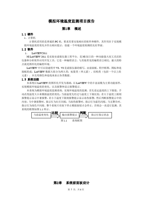
1.3 系统功能本系统以LabVIEW的图形化开发为基础,以LabVIEW中的丰富函数为主要功能部件,实现模拟环境温度的变化,以及报警和显示报警提示。
本系统为模拟环境温度监测系统,实现环境温度的监测。
首先设定温度的上下限值,手动改变温度大小来模拟温度的变化;当前温度先经过与温度上下限比较,若大于温度上限则报警提示显示中暑报警,若小于温度下限则报警提示显示冻伤报警;然后判断报警提示中的内容:当中暑报警时,指示灯为红灯闪烁;当冻伤报警时,指示灯为蓝色闪烁;当无警告时,指示灯为绿色不闪烁。
整个系统只有按下停止模拟按钮才会停止,否则会一直进行监测。
其系统的框图如图1.1所示。
图1.1 系统框图第2章系统前面板设计2.1 数值输入与显示控件在前面板中,使用了三个数值控件,在新式数值中可以找到。
其中两个数值输入控件,用来输入温度的上下限;一个数值显示控件,用来显示当前温度。
为了美观与方便,数值输入控件的显示项中去掉增量/减量;数值显示控件的属性中设置显示格式为浮点数、两位精度位数;把数值控件的标签均修改相应的提示信息,以便理解和观察。
2.2 垂直指针滑动杆垂直指针滑动杆在新式数值中,属于数值控件。
题目二PN结测温与模拟温度控制系统
1、设计要求
1.1 利用1N4148正向压降随温度线性变化的特性,测量温度并显示,精度0.5℃
1.2 通过键盘输入设定值,在温度的可控范围内控制功率电阻发热使之附近温度维持在设定温度
1.3 可以存储达到过的最高温度
2、要解决的关键问题及技术关键
2.1模拟量的采集调理,实现温度的测量。
2.2通过键盘输入设定值,在温度的可控范围内控制功率电阻发热使之附近温度维持在设定温度
2.3显示设定温度值和实际测量温度值。
2.4温控采用采用PID(比例积分微分调节器)+ PWM。
2.5 模拟加热可以采用图1电路,在PCB设计时1N4148贴近发热电阻即可。
3、解决途径
利用1N4148与电阻组成测温电桥,将电桥输出的差分电压送入三运放组成的仪表运放放大调理,再于A/D接口,利用单片机处理数据后显示。
采用PID算法与PWM控制结合的方式实现温度控制。
留出电桥输出端口,放大器输出端口,以便评估设计的模拟电路。
该电路可以用来模拟加热的过程,若IN处为
电平,则8550的e极导通,忽略管压降不计,流
过电阻电流I = 5/(5.1 + 5.1) = 0.5A,对于这样的
测量系统来说,这是很大的一个电流量。
经试验,
电阻发热量很大,在IN输输入PWM波即可实验
调温。
在测试的时候要注意供电电源的带负载能
力。
图1。
金属凝固过程计算机模拟题目:二维导热物体温度场的数值模拟Solidworks十字接头的传热分析作者:张杰学号:S2*******学院:北京有色金属研究总院专业:材料科学与工程成绩:2015 年12 月二维导热物体温度场的数值模拟图1 二维均质物体的网格划分用有限差分法模拟二维导热物体的温度场,首先将二维物体划分为如图1所示的网格,x ∆与y ∆可以是不变的常量,即等步长,也可以是变量(即在区域内的不同处是不同的),即变步长。如果区域内各点处的温度梯度相差很大,则在温度变化剧烈处,网格布得密些,在温度变化不剧烈处,网格布得疏些。至于网格多少,步长取多少为宜,要根据计算精度与计算工作量等因素而定。在有限的区域内,将二维不稳定导热方程式应用于节点,)i j (可写成: ,2222 ,i jPPp i j T T T C x y ρλτ⎛⎫∂∂∂=+ ⎪∂∂∂⎝⎭,1 , ,()i jP P Pi j i jT T T οτττ+-∂⎛⎫=+∆ ⎪∂∆⎝⎭ (), 1 , , 1 ,222()i j P P P Pi j i j i j T T T T x x x ο+--+∂⎛⎫=+∆ ⎪∂⎝⎭∆ () , ,1 , ,1222()i jPP P Pi j i j i j T T T T y y y ο+--+⎛⎫∂=+∆ ⎪∂∆⎝⎭τ∆、x ∆、y ∆ 当τ∆、x ∆、y ∆较小时,忽略()οτ∆、2()x ο∆、2()y ο∆项。
当x y ∆=∆时,即x 、y 方向网格划分步长相等。最后得到节点,)i j (的差分方程: ()1 , ,0 1 , 1 , ,1 ,1 ,4P P P P P P Pi j i j i j i j i j i j i j T T F T T T T T ++-+-=++++-式中:()02p F C x λτρ∆=∆。假设边界为对流和辐射边界,对流用以下公式计算:()(),1 , ,0 1 , ,1 ,1 ,24Pc f i j P P P P P P i j i j i j i j i j i j p a T T T T F T T T T C xτρ+-+-∆-=+++-+∆MATLAB 编程模拟clc; clear;format long %% 参数输入moni_canshu=xlsread('模拟参数输入.xlsx',1,'B2:B11'); %读取excel 中的模拟参数 s=moni_canshu(1); %几何尺寸,m t0=moni_canshu(2); %初始温度,℃tf=moni_canshu(3); %辐射(空气)边界,℃ rou=moni_canshu(4); %密度,kg/m3lamda=moni_canshu(5); %导热系数,w/(m ℃) Cp=moni_canshu(6); %比热,J/(kg ℃)n=moni_canshu(7); %工件节点数,个<1000 dt=60*moni_canshu(8); %时间步长,min to s m=moni_canshu(9); %时间步数,个<100 dx=s/(n-1);%计算dxf0=lamda*dt/(rou*Cp*dx*dx);%计算f0 %% 初始参数矩阵,初始温度 for iii=1:n for jjj=1:nTold(iii,jjj)=t0; end endTold(1,:)=tf; Told(n,:)=tf; Told(:,1)=tf;Told(:,n)=tf;%% 写文件表头xlswrite('data.xlsx',{['坐标位置']},'sheet1','A1');asc=97;for ii=1:nbiaotou1={['第' num2str(ii) '点']};asc=asc+1;xlswrite('data.xlsx',biaotou1,'sheet1',[char(asc) '1']);xlswrite('data.xlsx',biaotou1,'sheet1',['A' num2str(ii+1)]);end%% 模拟运算for jj=1:2copyfile('data.xlsx','data1.xlsx')Tnew(1,1:n)=tf;Tnew(n,1:n)=tf;Tnew(1:n,1)=tf;Tnew(1:n,n)=tf;for i=2:n-1for j=2:n-1Tnew(i,j)=Told(i,j)+f0*(Told(i-1,j)-4*Told(i,j)+Told(i+1,j)+Told(i,j-1)+Told(i,j+1)); endendTold=Tnew;pcolor(Told);%绘图shading interpcolormap(jet)pause(0.1)saveas(gcf,['第' num2str(jj*0.1) 's温度图像.jpg']);xlswrite('data1.xlsx',Told,'sheet1','B2');copyfile('data1.xlsx',['第' num2str(jj*0.1) 's数据.xlsx'])delete('data1.xlsx');end图3 模拟物体的温度分布图2 模拟物体的温度等高线图和温度梯度分布图。
模拟温度报警器课程设计一、课程目标知识目标:1. 学生能理解温度报警器的基本原理和模拟电路的组成。
2. 学生能掌握温度传感器的工作原理及其在报警器中的应用。
3. 学生能了解数字温度计的读数原理及其与模拟信号的转换方法。
技能目标:1. 学生能够运用所学知识,设计并搭建一个简单的模拟温度报警器电路。
2. 学生能够通过实验,熟练使用多用电表进行电路测试,并准确读取温度计数据。
3. 学生能够通过小组合作,进行电路调试和故障排查,提高问题解决能力。
情感态度价值观目标:1. 学生能够通过课程学习,培养对物理学科的兴趣,增强探究和实践的科学精神。
2. 学生在小组合作中,培养团队协作意识,学会相互尊重和倾听他人意见。
3. 学生能够认识到科技发明对生活的意义,培养创新意识和社会责任感。
课程性质:本课程为物理学科实验课,结合理论知识与动手实践,提高学生的综合运用能力。
学生特点:学生处于八年级,对物理现象有一定的好奇心,具备基本的电路知识和动手能力。
教学要求:通过本课程,教师应引导学生将理论知识与实际应用相结合,注重培养学生的动手实践能力和创新思维。
在教学过程中,关注学生的个体差异,鼓励学生积极参与,充分调动学生的学习积极性。
二、教学内容本课程教学内容主要包括以下三个方面:1. 理论知识:- 介绍温度传感器的基本原理,如热敏电阻的工作特性。
- 讲解模拟电路的组成,包括运算放大器、比较器等。
- 分析数字温度计的读数原理及与模拟信号的转换方法。
参考教材章节:第二章第三节“传感器及其应用”。
2. 实践操作:- 设计并搭建模拟温度报警器电路,包括温度传感器、运算放大器、比较器、指示灯等。
- 使用多用电表进行电路测试,学习测量温度传感器阻值、电压等参数。
- 小组合作进行电路调试和故障排查,确保温度报警器正常工作。
参考教材章节:第四章第二节“模拟电路的设计与搭建”。
3. 教学进度安排:- 第一课时:理论知识学习,介绍温度传感器和模拟电路原理。
温度场模拟matlab代码:clear,clc,clfL1=8;L2=8;N=9;M=9;% 边长为8cm的正方形划分为8*8的格子T0=500;Tw=100; % 初始和稳态温度a=0.05; % 导温系数tmax=600;dt=0.2; % 时间限10min和时间步长0.2sdx=L1/(M-1);dy=L2/(N-1);M1=a*dt/(dx^2);M2=a*dt/(dy^2);T=T0*ones(M,N);T1=T0*ones(M,N);t=0;l=0;k=0;Tc=zeros(1,600);% 中心点温度,每一秒采集一个点for i=1:9for j=1:9if(i==1|i==9|j==1|j==9)T(i,j)=Tw;% 边界点温度为100℃elseT(i,j)=T0;endendendif(2*M1+2*M2<=1) % 判断是否满足稳定性条件while(t<tmax+dt)t=t+dt;k=k+1;for i=2:8for j=2:8T1(i,j)=M1*(T(i-1,j)+T(i+1,j))+M2*(T(i,j-1)+T(i,j+1))+(1-2*M1-2*M2)*T(i,j);endendfor i=2:8for j=2:8T(i,j)=T1(i,j);endendif(k==5)l=l+1;Tc(l)=T(5,5);k=0;endendi=1:9;j=1:9;[x,y]=meshgrid(i); figure(1);subplot(1,2,1);mesh(x,y,T(i,j))% 画出10min 后的温度场 axis tight;xlabel('x','FontSize',14);ylabel('y','FontSize',14);zlabel('T/℃','FontSize',14) title('1min 后二维温度场模拟图','FontSize',18) subplot(1,2,2);[C,H]=contour(x,y,T(i,j)); clabel(C,H);axis square;xlabel('x','FontSize',14);ylabel('y','FontSize',14); title('1min 后模拟等温线图','FontSize',18) figure(2); xx=1:600;plot(xx,Tc,'k-','linewidth',2)xlabel('时间/s','FontSize',14);ylabel('温度/℃','FontSize',14);title('中心点的冷却曲线','FontSize',18)else disp('Error!') % 如果不满足稳定性条件,显示“Error !” end实验结果:时间/s温度/℃中心点的冷却曲线x1min后二维温度场模拟图T /℃xy1min 后模拟等温线图x5min 后二维温度场模拟图T /℃xy5min 后模拟等温线图x10min后二维温度场模拟图T /℃xy10min 后模拟等温线图x10min 后二维温度场模拟图(不满足稳定性条件)yT /℃21时间/s温度/℃中心点的冷却曲线(不满足稳定性条件)。
Journal of Materials Processing Technology 155–156(2004)1307–1312High temperature oxide scale characteristics of lowcarbon steel in hot rollingWeihua Sun ∗,A.K.Tieu,Zhengyi Jiang,Cheng LuFaculty of Engineering,University of Wollongong,North-fields Avenue,Wollongong,NSW 2522,AustraliaAbstractIn this paper,hot rolling tests of low-carbon steel were carried out on a 2-high Hille 100experimental rolling mill at various speeds and reductions.The rolling temperatures were between 1000and 1030◦C.Nitrogen protection was used to control the scale thickness when the test samples were heated in the furnace and cooled in a cooling box.The rolling forces,rolling torques and scale thicknesses before and after rolling were measured.Surface characteristics of the steel samples were analyzed with SEM and Atomic Force Microscope (AFM).X-ray diffraction was performed to characterize the phase composition of the scale layers.The effects of scale thickness on rolling force and torque were also investigated.©2004Elsevier B.V .All rights reserved.Keywords:Hot rolling;Oxide scales;Surface roughness1.IntroductionA scale layer is always formed on the strip surface dur-ing hot rolling process on a hot strip mill.Primary scales formed on the surface of slabs in the reheating furnace are removed by descaler.Secondary scale builds up again when the slab is waiting for further processing before each pass and before entering the finishing stands.Furthermore,tertiary oxidation scale layer develops after the slab is repeatedly descaled.Thus,the roll/strip interface in hot rolling always includes layers of scale.When the scale is subjected to rolling in the roll bite,it can act as a lubricant if it is thick and ductile,or as abrasives in the three-body wear mechanism if it is hard and brittle.Previous researches show that the oxide scale on the steel surface contains three layers:hematite,magnetite and wustite [1–3],even after any oxidation period longer than 0.6s [4].Each scale element has different morphology and mechanical properties [5,6].Tiley et al.[7]carried out hot compression tests on industrial reheating furnace scale of mild steel,indicating considerable plastic deformation when it was deformed at 30%strain with 0.1and 1.0s −1strain rate over the temperature range of 650–850◦C.Krzyzanowski and Beynon [8]conducted hot tension tests after producing scales of 10–300m in thickness and also found noticeable plastic deformation in the temperature∗Corresponding author.E-mail address:ws42@.au (W.Sun).range of 830–1150◦C.Yu and Lenard [9]estimated the re-sistance to deformation of the scale layer during hot rolling of carbon steel strips.However,little is known how the surface texture is trans-ferred from one pass to the next.It has been suggested that the texture is established by the work roll surface roughness during the rolling process [10].In the case of hot rolling,the actual surface texture is generated by a combination of the asperity contact and the lubricant contact between the strip and the roll.It was assumed that the scale is compressed and begins to be elongated when it enters the roll bite [11].When the oxide scale fractures and undertakes extreme pressure during rolling,the hot metal is extruded partially up into the fine cracks and hence modifying the strip surface roughness.The objective of the present work is to examine the effect of hot rolling parameters on the characteristics of the oxide scale of low carbon steel.The morphology of the scale and surface features of the strip before and after rolling was analyzed.Deformation behavior of the scale and its effects on the rolling force and torques were also examined.2.Experiment equipment,materials and procedures 2.1.EquipmentHot rolling experiments were carried out on a 2-high Hille 100experimental rolling mill with rolls of 225mm di-ameter and 254mm barrel roll,which is made of high speed steel (HSS)with a hardness of HRC55and R a of 0.4m in0924-0136/$–see front matter ©2004Elsevier B.V .All rights reserved.doi:10.1016/j.jmatprotec.2004.04.1671308W.Sun et al./Journal of Materials Processing Technology155–156(2004)1307–1312Table1Chemical composition of the steelElement Chemical composition(wt.%) C0.18Si0.18Mn0.95P0.026S0.027Cr0.10Ni0.067Cu0.13Mo0.19Al–T0.004Ti<0.003surfacefinishing.This rolling mill can operate at a rolling speed up to1m s−1,a load up to150t and a torque up to 13000kN m.It is equipped with two load cells to determine the compensations for the mill modulus and bearing clear-ance,and two torque gauges on the shaft to measure the individual roll torque.Two position transducers are used to control the roll gap.Two DMC-450radiation thickness gauges at entry and exit and a hydraulic AGC are available on the Hille100rolling mill.A Pentium III computer was used in the experiment.Its maximum sampling rate is250k s−1. In addition to the two optical pyrometers for controlling the surface temperature,a Flir PM390Thermo-camera by Thermoteknix Systems Limited was also used to measure the temperaturefield of the strip surface.Nitrogen was fed to the hearth of the reheating furnace in order to control the scale thickness and the steel bars were cooled in a box connected with nitrogen gas straight after rolling.A Nanoscope IIIA AFM from Digital Instruments and Leico E440SEM were used to analyze the topography of the strip surface.A Leico optical microscope and a Philips PW1730X-ray diffraction meter were also used characterize the morphologies and kinetics of the oxide scale.2.2.MaterialsThe test specimens were commercial low-carbon steel strip of dimension10mm×100mm in thickness and width. They were machined to9.20mm thickness,100mm width and450mm length.The surfaces were carefully prepared to0.5to0.7m in surfacefinishing,so that any influence of the original surface defects occurred from the industrial manufacturing could be prevented.Table1shows the chem-ical composition of the steel.2.3.Experiment procedureThe temperature of the furnace wasfirst raised to1100◦C and the nitrogen gas was then connected.Five minutes later, the test sample was put into the furnace hearth,waiting for the furnace temperature to reach1100◦C,the sample was soaked for10min to ensure uniform temperature.This pro-cedure took about23–25min.The sample was quickly rolled at1000◦C with a reduction from7.5to41%and rolling speeds between0.12and0.72m s−1.After rolling,the sam-ple were transferred into the cooling box which was con-nected to N2flow and aflow rate of20l min−1was selected. This rolling test was carried out one sample after another. The other series of tests were carried out in a similar proce-dure,but the furnace was not connected with N2and the steel samples were manually tapped to remove the oxide scale which was developed while soaking in the furnace.This is to remove the surface primary scale before rolling and to sim-ulate the descaling effect.There werefive or four samples heated each time for55–70or145–160min,respectively,to examine the effect of heating time on the behavior of the secondary scale under different deformation conditions. Samples for AFM,SEM and microscopic analysis were prepared from the rolled plates.3.Results and discussion3.1.Topography of the oxide scale before and after rolling As mentioned before,the steel surface is covered with a layer of oxide scale during hot rolling.Thus,the topology of the rolled steel product surface here is actually the topology of oxide scale.3D images of the steel surface after rolling can be seen from Fig.1(a)and(c).The samples were heated for60and65min of which the soaking period is for10 and15min,respectively.After they were extracted from the reheating furnace,manual descaling operation was carried out mechanically on the samples at the entry of the roll bite. About4–6s later,the samples were rolled.Then the samples were picked up at the exit of roll bite and stored in a cooling box,which was connected to N2flow.The total time taken from descaling to the cooling box were10.5–13s. Section analysis(Fig.1(b)and(d))was carried out along the rolling direction with Digital Nanoscope software ver-sion5.12b.As for the sample deformed at25%at the rolling speed of0.12m s−1,the maximum vertical distance between the peak and the valley,indicated with reversed triangles, was1.912m over a horizontal distance of6.45m(see Fig.1(b)).When the sample was deformed at33.7%at the rolling speed of0.12m s−1,the value of the maximum ver-tical distance was1.391m over a horizontal distance of 6.04m.These values seem to be much smaller than those in[12],which were obtained from simulated oxidizing tests on a Gleeble3500Thermo-Mechanical Simulator.As it will be discussed later,the total thickness of the scale on the descaled steel surface after rolling is<26m.Deformation effects could have an influence on the surface topology.A further examination of the surface morphology was conducted by scanning on the sample surface with SEM. Fig.2is the micrographs taken on the secondary oxide scale surfaces that were non-deformed,micrograph(a),and after deformed7.6%(Fig.2(b))and25%(Fig.2(c)),respectively,W.Sun et al./Journal of Materials Processing Technology 155–156(2004)1307–13121309Fig.1.3D image and section analysis of the rolled steel product surface:(a)and (b)after 25%deformation;(c)and (d)after 33.7%deformation.Rolling speed was 0.12m s −1.at the rolling speed of 0.12m s −1.On the non-deformed oxide scale surface,there are occasionally irregular long thin cracks,which are probably attributed by thermal-stress during cooling,see photo (a)in Fig.2.After deformation,short and coarse cracks appear transversely to the rolling direction (Fig.2(b)and (c)).These SEM micrographs reveal that visible plastic deformation the scale and the substrate have occurred.This is similar and consistent to the wear behavior which was observed by Vergne et al.[13].Fig.2(b)and (c)also show that the plastically deformed areas exhibit the extruded “under-cells”where the surfaces are oxidized.3.2.Deformation behavior of the oxide scale and morphological features of the secondary scaleMorphologies of the primary oxide scale were discussed in previous research [1–3,8,9].However,due to theirdiffer-Fig.2.Secondary oxide scale surface micrograph:(a)non-deformed;(b)and (c)deformed.ent mechanical properties,the scale may display a different behavior when deformed together with hot steel substrate by compression and tension.Fig.3illustrates the microstructures of the primary and secondary oxide scales before and after deformation.The samples for the test of primary oxide scale in Fig.3were heated one by one for about 23–25min each in the furnace.Results of the rolling test show that the primary scale exhibits its significant plastic deformation.Before deformation,the thickness of the scale turns out to be 297m,which is much larger than the values in [9,14].The reason could be that the heating time in [9,14]was much shorter than the present test.Cracks and large pores can be found in Fig.3(a).After it was deformed 15.8%at rolling speed of 0.12m s −1,the primary scale became 220m (Fig.3(b)).At the deformation of 33.7%when it was rolled at the speed of 0.48m s −1,the thickness was 127.7m (Fig.3(c)).This means that the scale1310W.Sun et al./Journal of Materials Processing Technology 155–156(2004)1307–1312Fig.3.Microstructures of the primary and secondary oxide scales before and after deformation:(a)and (d)non-deformed primary and secondary scale;(b)primary scale deformed 15.8%at rolling speed of 0.12m s −1;(c)primary scale deformed 33.7%at rolling speed of 0.48m s −1;(e)and (f)secondary scale deformed 15.8%at rolling speed of 0.24and 0.72m s −1,respectively.deformed 25.9%when the sample was subjected a 15.8%deformation and that it would deform 57%when the sample deformed 33.7%.There is a significant trend that the scale thickness decreases quickly with the bulk deformation.The rolling speeds also play a similar role on the thickness of the oxide scale (see Fig.4).Photos in Fig.3(d)–(f)are the microstructures for the sec-ondary oxide scales before and after deformation.The sam-ples were heated for 145–160min before it was descaled.The initial secondary scale thickness was 29.5m in this ex-periment.X-ray diffraction results show that there arethree Fig.4.Effects of reduction and rolling speed on the thickness of primary and secondary oxide scales.(a)Reductions from 7.6to 41.3%;(b)rolling speeds from 0.12to 0.72m s −1.components in the secondary layer,which are hematite,mag-netite and wustite.Magnetite shows its strongest presence at 2θ◦of 30.1,35.5,57.1and 62.6◦.However,hematite re-veals its significant presence at 33.1,35.7,49.5and 54.2◦even though it is shadowed by magnetite (Fig.5).From Fig.3(d),the interface between the scale and the substrate became rougher.Under a reduction of 15.8%,the scale thickness became 24and 24.2m,respectively,at rolling speeds of 0.24and 0.72m s −1.Although a 15.8%bulk deformation could reduce the thickness of the sec-ondary scale about 13.5%,the rolling speed does not seemW.Sun et al./Journal of Materials Processing Technology 155–156(2004)1307–13121311Fig.5.X-ray diffraction result of the secondary oxide scale.to have an effect on the secondary scale thickness (see Fig.4(b)).On the other hand,the bulk reduction does not have re-markable effects on the thickness of secondary scale (see Fig.4(a)).The samples were heated for 55–70min totally.The approximate thickness of the secondary scales were 10.9–11.4m after the samples were deformed 7.6,25and 33.7%at rolling speed of 0.12m s −1.This could be the reason that the total scale thickness was so small that the difference in scale thickness,which was caused by the deformation,could be compensated by oxidation while the sample was delivered to the cooling box.However,the re-sults of the test show another interesting outcome that the holding time of the samples will affect the secondary scale thickness significantly.The magnitude of the scale thick-ness value for 55to 70min heating time (Fig.4(a))is less than half of the value of the scales which were produced in 145–160min (Fig.4(b)).This implies that the thermal history of the steel in the furnace plays an important role on the oxide scale thickness even afterdescaling.Fig.6.Effects of reductions and rolling speeds on the surface roughness.3.3.Surface roughnessAfter rolling,surface roughness was measured to examine the effects of rolling parameters on the surface roughness.The results are shown in Fig.6.Bulk deformation affects significantly the surface finish of the sample surface.When the bulk deformation increases,the surface roughness decreases remarkably when oxide scale is thick (see Fig.6(a)).For the steel surface with pri-mary oxide scale,the surface roughness increases with re-duction at first.According to the present test,after reduction reached 15.8%,surface roughness decreases significantly with reduction.As for the descaled surfaces,the roughness decreases very quickly when reduction increases from 7.6to 25%.But when the bulk deformation increases further,the roughness reduction slows down.However,when there is a thin scale layer on the steel surface,the ability of deforma-tion to improve the surface roughness is impaired.On the other hand,the effect of rolling speeds on the surface roughness is complex in this experiment.In the case1312W.Sun et al./Journal of Materials Processing Technology155–156(2004)1307–1312of55–70min of heating,the roughness of both the descaled and non-descaled increases with rolling speed.On the other hand,the roughness decreases with increasing rolling speed when the sample heating time is145–160min.However, heavy reduction has a significant influence on the surface finish.4.ConclusionIn this paper,hot rolling tests were carried out on a Hille100mill.Topology and SEM analysis indicate that cracks occurred in the secondary oxide scale when sub-jected to bulk deformation and new“under-cell”extruded. Morphological examination shows that the primary ox-ide scale deforms when the bulk reduction increases or when the rolling speed increases at a certain reduction. However,an increase of bulk deformation or increase of rolling speed has limited influence in reducing the sec-ondary scale thickness.The secondary oxide scale is com-posed of three components similar to those for the primary scale.The thickness is greatly influenced by the heating history.More importantly,the bulk deformation has a sig-nificant effect on the surfacefinish of the hot rolled steel products.AcknowledgementsThis project is supported by an ARC-linkage grant.The first author would like to thank Australian Government for scholarship support(IPRS and UPA)to undertake this research.The authors are greatly thankful for the assis-tance from Dr.Hongtao Zhu while the rolling tests were carrying out.References[1]F.Matsuno,Blistering and hydraulic removal of scalefilms of rimmedsteel at high temperature,Trans.ISIJ.20(1980)413–421.[2]J.S.Sheasby,W.E.Boggs,E.T.Turkdogan,Scale growth on steelsat1200◦C:rationale of rate and morphology,Met.Sci.18(1984) 127–136.[3]I.Iordanova,M.Surtchev,K.S.Forcey,V.Krastev,High-temperaturesurface oxidation of low-carbon rimming steel,Surf.Interface Anal.30(2000)158–160;M.A.El Baradie,A fuzzy logic model for machining data selection, Int.J.Mach.Tools Manufact.37(1997)1353–1372.[4]Weihua Sun,A.K.Tieu,Zhengyi Jiang,Hongtao Zhu,Cheng Lu,Oxide scales growth of low carbon steel at high temperatures,in: Proceedings of AMPT2003,Dublin,8–11July2003(under review).[5]D.T.Blazevic,Tertiary rolled-in scale:the hot strip mill problem ofthe1990s,in:Proceedings of the37th MWSP Conference,ISS-AIME XXXVII(1996)33–38.[6]M.Schutze,An approach to a global model of the mechanicalbehaviour of oxide scales,Mater.High Temp.12(1994)237–247.[7]J.Tiley,Y.Zhang,J.G.Lenard,Hot compression testing of mildsteel industrial reheat furnace scale,Steel Res.70(1999)437–440.[8]M.Krzyanowski,J.H.Beynon,The tensile failure of mild steel oxideunder hot rolling conditions,Steel Res.70(1999)22–27.[9]Y.Yu,J.G.Lenard,Estimating the resistance to deformation of thelayer of scale during hot rolling of carbon steel strips,J.Mater.Proces.Technol.121(2001)60–68.[10]H.R.Le,M.P.F.Sutcliffe,Analysis of surface roughness of cold-rolledaluminium foil,Wear244(2000)71–78.[11]J.H.Beynon,Y.H.Li,M.Krzyzanowski, C.M.Sellars,Measur-ing modeling and understanding friction in hot rolling of steel,in: M.Pietrzyk et al.(Eds.),Proceedings of the Metal Forming2000, Balkema,Rotterdam,2000,pp.3–10.[12]W.Sun,A.K.Tieu,Z.Jiang,C.Lu,H.Zhu,Surface characteristicsof oxide scale in hot strip rolling,J.Mater.Proces.Technol.140 (2003)76–83.[13]C.Vergne,C.Boher,C.Levaillant,R.Gras,Analysis of the frictionand wear behavior of hot work tool scale:application to the hot rolling process,Wear250(2001)322–333.[14]A.Shirizly,J.G.Lenard,The effect of scaling and emulsion deliveryon heat transfer during the hot rolling of steel strips,J.Mater.Proces.Technol.101(2000)250–259.。