PFC手册例子耦合FLAC3D
- 格式:docx
- 大小:14.47 KB
- 文档页数:1
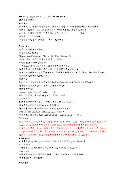
PFC3D 学习记录5-COMMAND REFERENCE通用规定和特征命令语法默认情况下,命令行忽略大小写,然而可以通过SET case命令激活区别大小写情况。
斜体字代表数字,以i, j, m n 为开头的字母代表整数,其他情况为实数命令词,关键字和数值可用空格,以及(),=分隔。
在分号(;)后为注释一行最多可包含80个字符。
而& 表示续行Range 语法定义一定限制范围的物体可运用Range的命令:Change/ initial/ property Clump Fix/ Free Group JsetModel Plot ( 运用于不同输出项目) PrintRange( 创建一个命名的范围)一个Range 定义一系列物体。
由许多范围元素构成。
如果使用多个范围元素,最终物体几何为不同元素集合的交集。
但是可通过关键词any改变选择特性。
如果使用关键词any选项,任何包含在范围内的单元可被认为最终物体集合的一部分。
即求合集除此之外,通过在定义范围单元后接关键词not确定所有不在指定范围的单元通常还可以用定义group 方式定义复杂的range。
内置范围单元:Annulus center ( x, y, z) radius = r1, r2球形空心区域中心在(x, y, z )内径r1, 外径r2Color il < iu >球体或墙体在间隔(il, iu )内颜色索引。
若无iu 则iu = il球体颜色索引列表通过property命令建立。
墙体颜色索引列表必须用FISH 内置的w_color设置Cylinder end1( x1, y1, z1 ) end2( x2, y2, z2 ) radius = r圆柱范围。
圆柱中心轴过end1( x1, y1, z1 ) end2( x2, y2, z2 ) 半径为r.Fish fname调用用户定义的范围单元。
通过FISH函数fname 执行。

FLAC3D流力耦合作用1. 1耦合作用简介 (1)1. 2数学模型描述 (2)1.2.1 规定和定义 (2)1.2.2 流体重量平衡方程 (3)1.2.3 流动法则 (4)1.2.4 力学结构法则 (4)1.2.5 边界及初始条件 (5)1. 3数值公式 (5)1.3.1空间导数的有限差分近似 (5)1.3.2质量平衡方程的节点公式 (6)1.3.3显式有限差分公式 (8)1.3.3.1稳定标准 (9)1.3.4隐式有限差分公式 (9)1.3.4.1收敛准则 (11)1.3.5力学时间步和力学稳定性 (12)1.3.6总应力修正 (12)1. 4流动耦合问题的属性和单位 (12)1.4.1 渗透系数 (13)1.4.2 Biot系数 和Biot模数M (13)1.4.3流体体积模量 (14)1.4.4孔隙率 (14)1.4.5密度 (14)1.4.6流体张力限 (15)1. 5单一流动问题和耦合流动问题 (15)1.5.1恒定孔压(用于有效应力计算) (15)1.5.2 建立了孔压分配的单一流动计算 (16)1.5.3 非流动,力学变形产生的孔隙压力 (16)1.5.4耦合流动和力学计算 (17)1. 6对于渗流分析的输入指导 (18)1.6.1 FLAC3D命令 (18)1.6.2 FISH变量 (21)1.7 验证举例 (22)1.7.1在限制层内的不稳定地下水流动 (22)1.7.2单方向固结 (25)1.7.3 穿透浅含水层限制边界的井水流动 (29)1.1耦合作用简介FLAC3D允许在饱和多孔材料中进行流体流动的瞬时模拟。
流动计算可以脱离FLAC 3D 中的力学计算独立进行,也可以与其他力学模型进行耦合计算,以控制流——固耦合作用的影响,其计算具有如下特征。
1. 提供了在各向同性条件下的流体运动法则,也提供了在流动区域中的无渗流材料的流动零模型。
2. 不同的区域可以有不同的流动模型和法则。
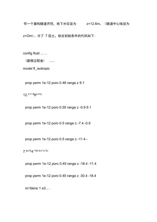
z=Om)。
分了7层土,给定初始条件的代码如下:config fluid A/ N( J8 c' l5 m; ~& z' P(建模过程省) . M7 P8 p6 S3 q8 c4model fl_isotropicprop perm 1e-12 poro 0.48 range z 9.112.3~7~$6p-h%|prop perm 1e-12 poro 0.55 range z -0.9 9.1 prop perm 1e-12 poro 0.5 range z -7.4 -0.9 prop perm 1e-12 poro 0.5 range z -11.4 -7.&u7S4~*|6n;S;c"cv"|Uprop perm 1e-12 poro 0.45 range z -18.4 -11.4prop perm 1e-12 poro 0.45 range z -30.4 -18.4ini fdens 1 e3:Y/b,u2 Y1 Y% i' cini fmod 8.5e7/R9 b7 a1 d* w " H) Y) aini sat 0 range z 12.6 15.1 ini sat 1 range z -30.4 12.62Q"e,q:|!n'Lini pp 0 grad 0 0 -1e4 range z -30.4 12.6'?'Q7k?6M7Q/h' hfix pp range x -.1 .1fix pp range x 39.9 40.1fix pp range y -.1 .1!b&R$ d* J @! C) X- Efix pp range y 119.9 1 20 . 14R+w6m8 B8 O- S, m+ {" B7 C8 m7 afix pp range z 12.5 12.7$M-V/~&N# s: vfix pp range z -30.5 -30.3;material mecha nic parameter'smodel mohr#g0V% u6 W, b. % f& }def derive+J:@6 d- I) F9 us_mod1=E_mod1/(2.0*(1.0+p_ratio1))b_mod1=E_mod1/(3.0*(1.0-2.0*p_ratio1))s_mod2=E_mod2/(2.0*(1.0+p_ratio2))b_mod2=E_mod2/(3.0*(1.0-2.0*p_ratio2))s_mod3二E_mod3/(2.0*(1.0+p_ratio3))•b_mod3二E_mod3/(3.0*(1.0-2.0*p_ratio3))s_mod4=E_mod4/(2.0*(1.0+p_ratio4))/}0 ]3 y/ H c: d; b3 h( qb_mod4=E_mod4/(3.0*(1.0-2.0*p_ratio4))s_mod5=E_mod5/(2.0*(1.0+p_ratio5))b_mod5=E_mod5/(3.0*(1.0-2.0*p_ratio5))s_mod6=E_mod6/(2.0*(1.0+p_ratio6))b_mod6=E_mod6/(3.0*(1.0-2.0*p_ratio6))s_mod7=E_mod7/(2.0*(1.0+p_ratio7))"{5 T/ R7 |, e) bb_mod7=E_mod7/(3.0*(1.0-2.0*p_ratio7))end (S/yset E_mod1=2.40e6 p_ratio1=0.25E_mod3=11.0e6 p_ratio3=0.25 &E_mod6=9.25e6 p_ratio6=0.22 &,X)zi* y E_mod7=12.40e6 p_ratio7=0.2deriveprop bulk b_mod5 shear s_mod5 cohe 18.0e3 fric 18.0 ten 55.398e3 range z 12.6 15.1prop bulk b_mod3 shear s_mod3 cohe 6.3e3 fric 21.0 ten 16.412e3 range z 9.1 12.6prop bulk b_mod1 shear s_mod1 cohe 13.2e3 fric 10.0 ten 74.861e3 range z 0 9.1)F%|6b7?,prop bulk b_mod1 shear s_mod1 cohe 13.2e3 fric 10.0 ten 74.861e3 E_mod2=5.0e6 p_ratio2=0.30 E_mod4=8.5e6 p_ratio4=0.25E_mod5=11.5e6 p_ratio5=0.27range z -0.9 0prop bulk b_mod2 shear s_mod2 cohe 15.3e3 fric 10.0 ten 86.771e3 range z -7.4 -0.9. Q* I5 S$ H2 x [prop bulk b_mod4 shear s_mod4 cohe 22.0e3 fric 20.0 ten 60.445e3 range z -11.4 -7.4&Q"o.d&W!n;q7 [7 Z4 x5 }prop bulk b_mod6 shear s_mod6 cohe 3.0e3 fric 25.0 ten 6.434e3 range z -18.4 -11.4prop bulk b_mod7 shear s_mod7 cohe 3.0e3 fric 25.0 ten 6.434e3 range z -30.4 -18.4;boundary conditions"Q# Z9 {% C7 Q $ ffix x range x -0.1 0.1fix x range x 39.9 40.1fix y range y -0.1 0.10N, A, u5 A( V& A/ ?. c( v" Jfix y range y 119.9 120.1fix x range z -30.5 -30.3…fix y range z -30.5 -30.3 # P8 F4 m8 X" \$ Nfix z range z -30.5 -30.3"m!L3g% }7 v$ Y$ V3 _interface 1 prop kn 3e9 ks 1e9 fric 20 coh 3e5interface 2 prop kn 3e9 ks 1e9 fric 20 coh 3e5;stress conditions;w(a3b-Z(P:x. {1 O' ]7 [, Kset grav 0 0 -10)W6j1h*}- ini dens 1.87e3 range z 12.6 15.1ini dens 1.87e3 range z 9.1 12.(K62F;l2e%v(}"X)r)|ini dens 1.76e3 range z 0 9.1$B9g3M1A ]! Eini dens 1.76e3 range z -0.9 0ini dens 1.84e3 range z -7.4 -0.! 9e&g9O;U-g7h;B8j4cini dens 2.0e3 range z -11.4 -7.24u%M"|;n2K0~8 ~7 Yini dens 1.89e3 range z -18.4 -11.4ini de ns 1.93e3 range z -30.4 -18.4ini szz -28.237e4 grad 0 0 1.87e4 range z 12.6 15.1 ini szz -28.237e4 grad 0 0 1.87e4 range z 9.1 12.6 ini szz -27.236e4 grad 0 0 1.76e4 range z 0 9.1ini szz -27.236e4 grad 0 0 1.76e4 range z -0.9" X+ M9 h/ }' m0(Zini szz -27.164e4 grad 0 0 1.84e4 range z -7.4 -0.9 ini szz -25.98e4 grad 0 0 2.0e4 range z -11.4 -7.4 ini szz -27.234e4 grad 0 0 1.89e4 range z -18.4 -114o5Z.!U-J-H$m4 ini szz -26.498e4 grad 0 0 1.93e4 range z -30.4 -18.4ini sxx -28.237e4 grad 0 0 1.87e4 range z 12.6 15.1 ini sxx -28.237e4 grad 0 0 1.87e4 range z 9.1 12.!p%c.D 6d3p!G7C0 z9 L ini sxx -27.236e4 grad 0 0 1.76e4 range z 0 9.1 ini sxx -27.236e4 grad 0 0 1.76e4 range z -0.9 , i' q8 l" c.0h$n.e;N ini sxx -27.164e4 grad 0 0 1.84e4 range z -7.4 -0.!Q;r:M:9Ji ini sxx -25.98e4 grad 0 0 2.0e4 range z -11.4 -7.4 ini sxx -27.234e4 grad 00 1.89e4 range z -18.4 -11.4 ini sxx -26.498e4 grad 0 0 1.93e4 range z -30.4 -18.4ini syy -14.905e4 grad 0 0 9.871e3 range z 12.6 157V..K"}2h7}/1s9W ini syy -13.597e4 grad 0 0 8.833e3 range z 9.1 12.6 ini syy -16.834e4 grad 0 0 1.239e4 range z 0 9.1 ini syy -16.834e4 grad 0 0 1.239e4 range z -0.9 0 ini syy -16.783e4 grad 0 0 1.296e4 range z -7.4 -0.4h.q!E9-~$]$D"K6q ini syy -19.117e4 grad 0 0 9.806e3 range z -11.4 -7.4;U-R)U5J;B!nv2D ini syy -21.550e4 grad 0 0 7.672e3 range z -18.4 -11.3_,z6_-H- 4@5d9f3] ini syy -21.252e4 grad 0 0 7.834e3 range z -30.4 -18.4(取控制点省) 4 Q/ a'h" K) |9 j2 S! tsolvesave iniconditions.sav初始平衡后的PP 如下图。
FLAC 3D基础知识介绍一、概述FLAC(Fast Lagrangian Analysis of Continua)由美国Itasca公司开发的。
目前,FLAC有二维和三维计算程序两个版本,二维计算程序V3.0以前的为DOS版本,V2.5版本仅仅能够使用计算机的基本内存64K),所以,程序求解的最大结点数仅限于2000个以内。
1995年,FLAC2D已升级为V3.3的版本,其程序能够使用护展内存。
因此,大大发护展了计算规模。
FLAC3D是一个三维有限差分程序,目前已发展到V3.0版本。
FLAC3D的输入和一般的数值分析程序不同,它可以用交互的方式,从键盘输入各种命令,也可以写成命令(集)文件,类似于批处理,由文件来驱动。
因此,采用FLAC程序进行计算,必须了解各种命令关键词的功能,然后,按照计算顺序,将命令按先后,依次排列,形成可以完成一定计算任务的命令文件。
FLAC3D是二维的有限差分程序FLAC2D的护展,能够进行土质、岩石和其它材料的三维结构受力特性模拟和塑性流动分析。
调整三维网格中的多面体单元来拟合实际的结构。
单元材料可采用线性或非线性本构模型,在外力作用下,当材料发生屈服流动后,网格能够相应发生变形和移动(大变形模式)。
FLAC3D采用的显式拉格朗日算法和混合-离散分区技术,能够非常准确的模拟材料的塑性破坏和流动。
由于无须形成刚度矩阵,因此,基于较小内存空间就能够求解大范围的三维问题。
三维快速拉格朗日法是一种基于三维显式有限差分法的数值分析方法,它可以模拟岩土或其他材料的三维力学行为。
三维快速拉格朗日分析将计算区域划分为若干四面体单元,每个单元在给定的边界条件下遵循指定的线性或非线性本构关系,如果单元应力使得材料屈服或产生塑性流动,则单元网格可以随着材料的变形而变形,这就是所谓的拉格朗日算法,这种算法非常适合于模拟大变形问题。
三维快速拉格朗日分析采用了显式有限差分格式来求解场的控制微分方程,并应用了混合单元离散模型,可以准确地模拟材料的屈服、塑性流动、软化直至大变形,尤其在材料的弹塑性分析、大变形分析以及模拟施工过程等领域有其独到的优点。
Flac3D中文手册Flac3D 中文手册FLAC3D的计算模式中是否需要做孔压分析取决于是否采用config fluid命令。
1 无渗流模式(不使用config fluid)即使不使用命令config fluid,仍然可以在节点上施加孔压。
这种模式下,孔压将保持为常量。
如果采用塑性本构模型的话,材料的破坏将由有效应力状态来控制。
节点上的孔压分布可由initial pp命令或water table命令来设定。
如果采用water table命令,由程序自动计算水位线以下的静水孔压分布。
此时,必须施加流体密度(water density)和重力(set gravity)。
流体密度值和水位位置可以用命令print water显示。
如果水位线是由face关键字来定义的,则可用命令plot water命令显示水位。
这两种情况,单元的孔压都由节点孔压值平均求出,并在本构模型计算中用作有效应力。
这种计算模式下,体积力中不反映流体的出现:用户必须根据水位线以上或以下相应地指定干密度和湿密度。
使用命令print gp pp和priint zone pp可分别得到节点或单元孔压。
plot contour pp命令可绘出节点孔压云图。
2 渗流模式(使用config fluid)如果使用命令config fluid,则可进行瞬时渗流分析,孔压改变和潜水面的改变都可能出现。
在config fluid模式下,有效应力计算(静态孔压分布)和非排水计算均被执行。
除此之外,还可进行全耦合分析,这种情况下,孔压改变将使固体产生变形,同时体积应变反过来影响孔压的变化。
如果采用渗流模式,单元孔压仍由节点孔压平均求出。
但这种模式,用户只能指定干密度(不论是水位以上还是以下),因为FLAC3D 将流体的影响考虑到了体积力的计算中。
采用渗流模式时,渗流模型必须施加到单元上,使用命令model fl_isotropic模拟各向同性渗流,model fl_anisotropic模拟各向异性渗流,model fl_null模拟非渗透物质。
FLAC/FLAC3D常规问题的整理1.FLAC3D命令的FAQlakewater整理看到其它板块上都有这个FAQ,也就是常见问题问答,今天抽了时间进行了整理,想到了就写下来了,因为看到很多初学者费了很多的时间,但是还是没有将常用的命令掌握,所以这个也可以作为入门的初级教材,使大家能够快速的上手,而不用为了某个小命令到处求助。
1. FLAC3D是有限元程序吗?答:不是!是有限差分法。
2. 最先需要掌握的命令有哪些?答:需要掌握gen, ini, app, plo, solve等建模、初始条件、边界条件、后处理和求解的命令。
3. 怎样看模型的样子?答:plo blo gro可以看到不同的group的颜色分布4. 怎样看模型的边界情况?答:plo gpfix red sk5. 怎样看模型的体力分布?答:plo fap red sk6. 怎样看模型的云图?答:位移:plo con dis (xdis, ydis, zdis)应力:plo con sz (sy, sx, sxy, syz, sxz)7. 怎样看模型的矢量图?答:plo dis (xdis, ydis, zdis)8. 怎样看模型有多少单元、节点?答:plo info9. 怎样输出模型的后处理图?答:File/Print type/Jpg file,然后选择File/Print,将保存格式选择为jpe文件10. 怎样调用一个文件?答:File/call或者call命令10. 如何施加面力?答:app nstress11. 如何调整视图的大小、角度?答:综合使用x, y, z, m, Shift键,配合使用Ctrl+R,Ctrl+Z等快捷键12. 如何进行边界约束?答:fix x ran (约束的是速度,在初始情况下约束等效于位移约束)13. 如何知道每个单元的ID?答:用鼠标双击单元的表面,可以知道单元的ID和坐标14. 如何进行切片?答:plo set plane ori (点坐标) norm (法向矢量)plo con sz plane (显示z方向应力的切片)15. 如何保存计算结果?答:save +文件名16. 如何调用已保存的结果?答:rest +文件名;或者File / Restor17. 如何暂停计算?答:Esc18. 如何在程序中进行暂停,并可恢复计算?答:在命令中加入pause命令,用continue进行继续19. 如何跳过某个计算步?答:在计算中按空格键跳过本次计算,自动进入下一步20. Fish是什么东西?答:是FLAC3D的内置语言,可以用来进行参数化模型、完成命令本身不能进行的功能21. Fish是否一定要学?答:可以不用,需要的时候查Mannual获得需要的变量就可以了22. FLAC3D允许的命令文件格式有哪些?答:无所谓,只要是文本文件,什么后缀都可以23. 如何调用一些可选模块?答:config dyn (fluid, creep, cppudm)后注:这个工作很繁琐,需要的时间很多,希望广大网友能够将自己曾经遇到的常见问题在后续跟贴,也为了将这个FAQ进行很好的充实。
第43卷第5期2 0 2 1年5月铁 道 学 报JOURNAL OF THE CHINA RAILWAY SOCIETYVol.43 No.5May 2 0 2 1文章编号:1001-8360(2021)05-0144-09基于PFC ・FLAC 耦合的弹性轨枕力学特性分析崔旭浩,肖宏(北京交通大学轨道工程北京市重点实验室,北京100044)摘要:采用离散单元法建立了具有棱角特征的精细化道床模型,采用有限差分法建立了可考虑变形的连续介质 轨枕模型,推导了组合道砟颗粒与有限差分单元之间的接触位移关系,通过在轨枕与道床之间设置耦合边界进行力和位移的交互实现二者的耦合计算,依据现场实测结果验证了模型的正确性。
对建立的弹性轨枕有砟道床和普通轨枕有砟道床施加动荷载,对比两者的计算结果发现:弹性轨枕可以增大轨枕底面与散体道砟之间的接触面积,减小接触应力;弹性轨枕可以有效减少道床顶层范围内道砟颗粒之间较大接触力的岀现;弹性轨枕可以降低 道床内部道砟颗粒之间的平均接触力和最大接触力;道砟颗粒之间接触力的概率密度随着接触力的增大而逐渐减小,铺设弹性轨枕可以减低道床内部较大接触力岀现的概率,起到保护道砟的作用;弹性轨枕可以减小道床的振动加速度;从控制轨枕-道床结构的振动水平和道床的弹性变形量等角度综合考虑,建议枕下胶垫的合理静刚 度取值为70〜100 kN/mm 。
关键词:有砟道床;弹性轨枕;PFC-FLAC 耦合;力学特性中图分类号:U213. 3文献标志码:A doi : 10. 3969/j.issn.l001-8360. 2021. 05. 017Mechanical Characteristics Analysis of Elastic Sleeper Based onPFC-FLAC Coupling MethodCUI Xuhao, XIAO Hong(Beijing Key Laboratory of Track Engineering , Beijing Jiaotong University , Beijing 100044 , China)Abstract : A refined ballast bed model with angular features was established based on discrete element method. The fi nite-difference method was used to establish a continuum-sleeper model that considers deformation. The contact displace ment relationship between the composite ballast particles and the finite difference element was derived. The coupling model was established by setting the coupling boundary between sleeper and ballast bed to exchange forces and displace ments. The correctness of the model was verified by field test results. The ballast bed model with elastic sleeper and ordi nary sleeper was applied with dynamic load. The results show that the elastic sleeper can increase the contact area be tween the sleeper bottom and ballast bed and reduce the contact stress. Elastic sleeper can effectively reduce the occur rence of large contact force between ballasts in the top layer of ballast bed, and can reduce the average contact force and the maximum contact force between ballasts. The probability density of the contact force between ballasts decreases with the increase of contact force. Laying elastic sleepers can reduce the occurrence probability of large contact forces inside the ballast bed and protect the ballasts. Elastic sleeper can reduce the acceleration of ballast. The proper static stiffnessvalue of sleeper pads was suggested to be from 70 to 100 kN/mm with the comprehensive consideration of the sleeper ac celeration, ballast bed acceleration and the elastic deformation of ballast bed.Key words : ballast bed ; elastic sleeper ;PFC-FLAC coupling ; mechanical properties轨相互作用不断加剧,散体道床在剧烈振动下越发容易出现道祚破碎、粉化等劣化现象,这不仅增大了工务养护维修工作量,还会产生道床板结等影响行车安全,因此采取有效的措施减小道祚破碎、粉化是十分必要的。

与FLAC3D 的2.0和2.1版本相比,FLAC3D 3.0有哪些新功能?答:计算方面:1.所有的计算和数据均采用双精度浮点制。
2.其运行速度较2.1约快10-15%功能方面:1. 动力模块中增加了hysteretic阻尼对于动力计算,加入了一个新的阻尼特性:hysteretic阻尼。
采用这种形式的阻尼,数值计算模拟产生的应变可基于模型模量和阻尼函数的共同作用。
这就可以使用户将等价线性计算方法的结果与完全非线性无折减本构模型的计算结果进行比较。
另外,对一些其它形式的阻尼,如Rayleigh阻尼,进行了较大的折减,这样在使用hysteretic 阻尼时可以有效地节省计算时间。
2. 在岩石本构模型中增加了Hook-Brown(霍克-布朗)模型加入了霍克-布朗屈服准则,使用户对岩石材料计算结果较为合理。
它的屈服面是非线性的,同时是考虑最大、最小主应力的关系的基础上产生的。
该模型综合了塑性流准则,其特性随着不同的应力水平,呈一变化的函数。
3.热/流体水平对流模型FLAC3D之前已经能提供非线性固体与多孔介质渗流的流固耦合模拟,机械地耦合流体和固体。
而3.0版本的新功能增加了温度可受流体密度影响和流体中温度的水平对流。
4. 3Dshop生成的网格导入3DSHOP是一种能力强大的固体建摸和六面体网格的软件包,也是ITASA的产品。
FLAC3D 原始的网格仍可用,但是用基于WINDOWS操作系统的3DSHOP建复杂模型更为简单方便。
3DSHOP生成的网格能被FLAC直接读取。
5. 动画命令:FLAC3D现在能产生AVI和DCX动画,这是以前的版本没有的功能。
6. 记录颗粒轨迹:颗粒的路径能被记录和显示此外,FLAC3D 3.0也包含下面的新特点(这也是以前版本所不能实现的):1)网络版2)应用于混凝土加工模拟的水合作用模型。
问:如何显示变形轮廓线的命令?答:plo ske magf 10 其中10为放大系数问:如何查看各个时段不平衡力的具体数值?答:采用his来记录计算,包括位移应力等命令his unbalhis gp(zone) zdis range (0 0 0) 或者id=?导出数据命令his write n vs m begin 时步 end 时步 file filename.hisn表示纪录的id m表示时步要导出不平衡力的具体数值his unbalstep 100000 or solvehis write 1 vs step begin 1 end 1000 file 123.his使用上述命令就可以查看各个时步下的不平衡力的具体数值问:initial 与 apply 有何区别?答:initial初始化命令,如初始化计算体的应力状态等;apply边界条件限制命令,如施加边界的力、位移等约束等。
陈老师好,请问flac能模拟地裂缝吗?还有就是断层的上下2盘该怎么融合呢?答地裂缝问题很难,因为FLAC本身是连续介质的理论。
回复收起回复2楼2013-06-21 00:25举报|个人企业举报垃圾信息举报本楼含有高级字体我也说一句若惜青吧主12问陈教授您好,FLAC作动力分析采用的吸收边界效果怎么样,不知您是否关注过?答效果很好啊,欢迎使用。
我就是做动力分析的回复收起回复3楼2013-06-21 00:26举报|个人企业举报垃圾信息举报本楼含有高级字体我也说一句若惜青吧主12问老师你好还是设置SHELL单元的问题主要由于表面不规则范围不知道怎么确定比如要在刷坡体表面设置shell 该怎么设定范围答不规则没有关系,你只要找到正确的range,程序会自动识别这个range范围内所有的“面”,就可以建立正确的shell了。
问最大最小主应力迹线用哪个命令显示呢?用箭线的方向和长度反应应力的大小和方向答plot stensor陈老师您好隧道开挖后的最大最小主应力云图有什么作用呢答有助于判断周围土体的应力状态,包括大主应力方向,了解应力集中的区域,以应对周围土体破坏等工程问题。
问现在的研究生论文貌似都多多少少有点数值模拟,很多是不用模拟都知道结果的,这...答“多多少少”、“很多”,概念太模糊。
既然你已经知道这样,所以你应该选择一些未知的、有重要意义的问题来做数值模拟,ok?问再问陈老师,在模拟深部构造应力时,除了您书上说的SB法外,我个人想了一个思路:即模型四周加构造应力边界条件,底面固定,顶面施加一个应力边界条件来反演埋深自重应力,这样计算可以吗?答是否可行,一试便知。
有新想法很好,但是要对该方法的正确性进行验证方可。
问陈老师,您好!在您的PPT中提及:接触面有三种工作模式-粘结界面、粘接滑移、库仑滑移。
请问,在命令流中,分别控制哪个参数;其工作原理又是怎样的,谢谢!答1、三种模式主要是根据接触面参数来确定的,建模的命令都一样,但是参数赋值不同。
FLAC3D手册部分例题代码Example 8.1 BEAM PM.DATDEF _variables; geometry_length = 10.0_nbeam = 20; plastic bending moment_Mp = 50.0_negMp = -_Mp; iteration procedure_w_min = 5.5_w_max = 6.5_w_incr = 0.05_limit_step = 100000_root_fsave = ’beam_respm’; computed variables_nnode = 2_del_length = float(_length/_nbeam)END_variablessel beam begin=(0.0, 0.0, 0.0) end=(_length, 0.0, 0.0) nseg=_nbeam; beam propertiessel beam prop emod=210e3 nu=0.3sel beam prop XCArea=1.0 XCIy=0.083 XCIz=0.083 XCJ=1.25e-4 pmom _Mp ; fix b.c. for external nodessel node fix x y z xr zr range id=1sel node fix y z xr zr range id=2; apply bending momentsel node apply mom= (0 _negMp 0) range id=1;set mec step=_limit_stepDEF _find_w_crit_flag_continue = 1_accum_cycles = 0_load = _w_minz_load = - _load_counter = 1loop while _flag_continue = 1commandhistory resethis id=10 unbalhis id=20 sel node xdisp id= _nnodehis id=21 sel node xvel id= _nnodehis id=30 sel node ydisp id= _nbeamhis id=31 sel node yvel id= _nbeamsel beam apply zdist z_loadsolve ratio 1.0e-5 ;end_command_solve_cycles = step - _accum_cycles_accum_cycles = _accum_cycles + _solve_cycles_filename = _root_fsave + ’_’ + string(_counter)+’.sav’commandsave @_filenameend_command_line = ’Load = ’+st ring(_load)_out = out(_line)_line = ’Case just solved is STABLE ...’if _solve_cycles = _limit_step_flag_continue = 0 ; cycles reached limit (unstable case)_line = ’Case just solved is UNSTABLE (maximum steps reached)...’else_load = _load + _w_incrz_load = - _loadif _load > _w_max_flag_continue = 0_line = ’Case just solved is STABLE and the LAST one...’end_ifend_if_out = out(_line)_line = ’Case stored in file: ’+_filename_out = out(_line)_counter = _counter + 1end_loopENDset log on_find_w_critset log offreturnWheel Load over a Buried Pipe.DATgen zon radcyl p0 0,0,0 p1 3.4,0,0 p2 0,1,0 p3 0,0,3.4 &p4 3.4,1,0 p5 0,1,3.4 p6 3.4,0,3.4 p7 3.4,1,3.4 &p8 2,0,0 p9 0,0,2 p10 2,1,0 p11 0,1,2 &size 5 2 8 3gen zon radcyl p0 0,0,0 p1 0,0,-2.4 p2 0,1,0 p3 3.4,0,0 &p4 0,1,-2.4 p5 3.4,1,0 p6 3.4,0,-2.4 p7 3.4,1,-2.4 &p8 0,0,-2 p9 2,0,0 p10 0,1,-2 p11 2,1,0 &size 5 2 8 3gen zone brick p0 3.4,0,0 p1 7,0,0 p2 3.4,1,0 p3 3.4,0,3.4 &size 6 2 4 rat 1.1gen zone brick p0 3.4,0,-2.4 p1 7,0,-2.4 p2 3.4,1,-2.4 p3 3.4,0,0 & size 6 2 4 rat 1.1gen zone reflect norm 0,-1,0 ori 0,1,0gen zone reflect norm 0,-1,0 ori 0,2,0gen zon radcyl p0 0,4,0 p1 3.4,4,0 p2 0,12,0 p3 0,4,3.4 &p4 3.4,12,0 p5 0,12,3.4 p6 3.4,4,3.4 p7 3.4,12,3.4 &p8 2,4,0 p9 0,4,2 p10 2,12,0 p11 0,12,2 &size 5 6 8 3 ratio 1 1.2gen zon radcyl p0 0,4,0 p1 0,4,-2.4 p2 0,12,0 p3 3.4,4,0 &p4 0,12,-2.4 p5 3.4,12,0 p6 3.4,4,-2.4 p7 3.4,12,-2.4 &p8 0,4,-2 p9 2,4,0 p10 0,12,-2 p11 2,12,0 &size 5 6 8 3 ratio 1 1.2gen zone brick p0 3.4,4,0 p1 7,4,0 p2 3.4,12,0 p3 3.4,4,3.4 &size 6 6 4 rat 1.1 1.2gen zone brick p0 3.4,4,-2.4 p1 7,4,-2.4 p2 3.4,12,-2.4 p3 3.4,4,0 & size 6 6 4 rat 1.1 1.2model mohrini dens 2.0set grav 0 0 -10prop bulk 65000 she 30000prop coh 5.0 fric 34 ten 1.0 dil 20set largefix x y z range z -2.5 -2.3fix x range x -.1 .1fix x range x 6.9 7.1fix y range y -.1 .1fix y range y 11.9 12.1;hist unbalhist gp zdisp 0,1.0,3.4hist gp zdisp 0,1.0,2save pipe_geo.sav;; add pipesel shell range cyl end1 0 0 0 end2 0 12 0 rad 2sel shell prop iso 227e6 0.25 thick 0.012sel node fix y xr zr range y -.1 .1sel node fix y xr zr range y 11.9 12.1sel node fix x yr zr range x -.1 .1solvesave pipe_ini.savini xdis 0.0 ydis 0.0 zdis 0.0; apply wheel load at surfaceapply zvel -2.5e-5 range x -.1 .90 y 0.9 1.6 z 3.3 3.6 def p_loadload_head = nullpnt = gp_headloop while pnt # nullif gp_zpos(pnt) > 3.3 thenif gp_xpos(pnt) < 0.90 thenif gp_ypos(pnt) < 1.6 thenif gp_ypos(pnt) > 0.9 thenmpnt = get_mem(2)mem(mpnt) = load_headmem(mpnt+1) = pntload_head = mpntendifendifendifendifpnt = gp_next(pnt)endloopendp_load;def w_loadpnt = load_headwload = 0.0loop while pnt # nullwload = wload + gp_zfunbal(mem(pnt+1))pnt = mem(pnt)endloopw_load = wload / 0.40endhist w_loadhist gp zdisp 0,1.0,3.4step 6000save pipe_ld.sav; stress recovery ...sel recover surf surfx 1 2 3def z_dfishz_d = 0.006endz_dfishsel recover stress depth_fac z_ddef misesmax_mises = 0.0pnt_se = s_headloop while pnt_se # nully_pos = s_pos(pnt_se,2)if y_pos < 2.0 thensig_xx = sst_str(pnt_se,0,1)sig_yy = sst_str(pnt_se,0,2)sig_zz = sst_str(pnt_se,0,3)sig_xy = sst_str(pnt_se,0,4)sig_yz = sst_str(pnt_se,0,5)sig_xz = sst_str(pnt_se,0,6)mstr = (sig_xx + sig_yy + sigzz) / 3.dsxx = sig_xx - mstrdsyy = sig_yy - mstrdszz = sig_zz - mstrdsxy = sig_xydsyz = sig_yzdsxz = sig_xzvmstr2 = 1.5 * (dsxx*dsxx + dsyy*dsyy + dszz * dszz)vmstr2 = vmstr2 + 3. * (dsxy * dsxy + dsys * dsyz + dsxz * dsxz) if vmstr2 > 0.0 thensr_vmstr = sqrt(vmstr2)elsesr_vmstr = 0.0endifmax_mises = max(max_mises,sr_vmstr)endifpnt_se = s_next(pnt_se)endloopendmisesprint max_misesretFLAC手册部分例题代码A Shallow Tunnel in Soft Ground.dat; It's good manners to allow for extra arrays for use in FISH. In this; case it is expected that only five will be needed - but who knows!config extra 10; Register the generic FISH functions - must be done prior to their usecall fishtank.fis; set the number of ij zonesgrid 120 45mod mo; Make the ij grid fit 120m by 45m with origin at surface above tunnel center gen -60,-45 -60,0 60,0 60,-45; Mark the circle representing the tunnel and map the marked points to; extended array number 3 for later retrievalgen circ 0 -15 3ini ex_3 1 mark; Mark the sloping horizonini x=-60 y=-11 i= 1 j=35ini x= 50 y= 0 i=111 j=46gen line -60 -11 50 0ini y 0 j 46; initial stressini syy -8.55e5 var 0 8.55e5ini sxx -5.13e5 var 0 5.13e5ini szz -6.00e5 var 0 6.00e5; turn gravity onset g 10; boundary conditions - pick either pressure or displacement; don't forget to select appropriate lines as shown later in file; PRESSURE - fix x y bottom and apply pressure boundaries on sidesfix x y j 1app sxx -5.13e5 var 0 5.13e5 i 1app sxx -5.13e5 var 0 5.13e5 i 121; DISPLACEMENT - fix x y bottom and x on sides; fix x y j 1; fix x i 1; fix x i 121; material propertiespro bulk 13.333e6 she 8.000e6 fric 27 coh 1e10 ten 1e10 dil 0 den 1900pro bulk 41.667e6 she 19.231e6 den 2000 reg 1 45pro fric 35 coh 1e10 ten 1e10 dil 5 reg 1 45; get histories of unbalanced forces and vertical movement at surface above tunnelhist unbalhist ydisp i=61, j=46; initialize elastic stress statestep 4998; check equilibriumplot his 1plot his 2; reset material properties to actual valuesprop coh 2e4 tens 1e4prop coh 0 tens 0 reg 1 45step 1 ; still in equilibrium if unbalanced force does not increase; clean up displacement records in modelini xd 0 yd 0; save initial stress state - pick names according to boundary conditions ; don't forget to select appropriate lines as shown later in file; PRESSURE boundarysave g1p.sav; DISPLACEMENT boundary; save g1d.sav; Relaxation logic is based on marked gridpoints; Remove marked gridpoints that are not in the excavation boundary unmarkget_marks_back; dig out tunnelmode null reg 60 30; define closure histories as FISH functions; horizontal closure of tunneldef hcloshclos = xdisp(58,31)-xdisp(64,31)end; vertical closure of tunneldef vclosvclos = ydisp(61,28) - ydisp(61,34)end; replace tunnel core with equivalent tractionsfix x y marstep 1find_rffree x y marhist relaxhist hcloshist vcloshist ydisp i 61 j 46; set parameters for relaxation function 'calc'set np 20 k_ini 1 ; relaxation in 5% increments; for ground reaction curve do not save intermediate stateset relaxsave = 0; after initial runs to find ground reaction curve repeat analysis to select relaxation; point at which lining is to be installed - we decide to use 60% relaxation; results will be stored in g1p12.sav for PRESSURE boundary; set relaxsave = 0.60 fname 'g1p'; results will be stored in g1d12.sav for DISPLACEMENT boundary; set relaxsave = 0.60 fname 'g1d'; calculate ground reaction curvecalc; save calculations - pick names according to boundary conditions; don't forget to select appropriate lines as shown later in file; save PRESSURE boundary calculationsave g1p_gr.sav; save DISPLACEMENT boundary calculation; save g1d_gr.sav; plot and record results for ground reaction plotplot hist 4 5 -6 vs 3 beg 5000 end 35000 skip 200hist write 4 5 -6 vs 3 begin 5000 skip 200ret; install lining in tunnel at 60% relaxation - pick names according to boundary conditions ; don't forget to select appropriate lines as shown later in file; PRESSURE boundary runrest g1p12.sav; DISPLACEMENT boundary run;rest g1d12.sav; remove reaction forces from tunnelset relax=1.0app_rf; install lining using FISH function from FISH library (the FISH volume)ca beam.fisset ib=58 jb=30 ie=64 je=30beam; lining properties representing shotcretestru pro 1 e 21e9 a .1 i 83.33e-6step 4000; save lining results - pick names according to boundary conditions; that's all the changes; save PRESSURE boundary resultssave g1pshot.sav; save DISPLACEMENT boundary results; save g1dshot.sav; Linearly graded mesh - PRESSURE and DISPLACEMENT boundaries; Go through file and comment out appropriate lines as indicated; reset FLACnew; It's good manners to allow for extra arrays for use in FISH. In this; case it is expected that only five will be needed - but who knows!config extra 10; Register the generic FISH functions - must be done prior to their usecall fishtank.fis; set the number of ij zonesgrid 86 31mod mo; Make the ij grid fit 120m by 45m with origin at surface above tunnel center gen -60,-45 -60,-20 -30,-12 -30,-45 i= 1,14 j= 1,12 rat 0.9009,0.8850gen same -60, 0 -30, 0 same i= 1,14 j=12,32 rat 0.9009,1.0000gen same same 30,-20 30,-45 i=14,74 j= 1,12 rat 1.0000,0.8850gen same same 30, 0 same i=14,74 j=12,32gen same same 60,-20 60,-45 i=74,87 j= 1,12 rat 1.1100,0.8850gen same same 60, 0 same i=74,87 j=12,32 rat 1.1100,1.0000; Mark the circle representing the tunnel and map the marked points to; extended array number 3 for later retrievalgen circ 0 -15 3ini ex_3 1 mark; Mark the sloping horizonini x=-60 y=-11 i= 1 j=21ini x= 50 y= 0 i=84 j=32gen line -60 -11 50 0ini y 0 j 32; initial stressini syy -8.55e5 var 0 8.55e5ini sxx -5.13e5 var 0 5.13e5ini szz -6.00e5 var 0 6.00e5; turn gravity onset g 10; boundary conditions - pick either pressure or displacement; don't forget to select appropriate lines as shown later in file; PRESSURE - fix x y bottom and apply pressure boundaries on sidesfix x y j 1app sxx -5.13e5 var 0 5.13e5 i 1app sxx -5.13e5 var 0 5.13e5 i 87; DISPLACEMENT - fix x y bottom and x on sides; fix x y j 1; fix x i 1; fix x i 87; material propertiespro bulk 13.333e6 she 8.000e6 fric 27 coh 1e10 ten 1e10 dil 0 den 1900pro bulk 41.667e6 she 19.231e6 den 2000 reg 1 31pro fric 35 coh 1e10 ten 1e10 dil 5 reg 1 31; get histories of unbalanced forces and vertical movement at surface above tunnel hist unbalhist ydisp i=44, j=32; initialize elastic stress statestep 4998; check equilibriumplot his 1plot his 2; reset material properties to actual valuesprop coh 2e4 tens 1e4prop coh 0 tens 0 reg 1 31step 1 ; still in equilibrium if unbalanced force does not increase; clean up displacement records in modelini xd 0 yd 0; save initial stress state - pick names according to boundary conditions; don't forget to select appropriate lines as shown later in file; PRESSURE boundarysave g2p.sav; DISPLACEMENT boundary; save g2d.sav; Relaxation logic is based on marked gridpoints; Remove marked gridpoints that are not in the excavation boundaryunmarkget_marks_back; dig out tunnelmode null reg 43 16; define closure histories as FISH functions; horizontal closure of tunneldef hcloshclos = xdisp(41,17)-xdisp(47,17)end; vertical closure of tunneldef vclosvclos = ydisp(44,14) - ydisp(44,20)end; replace tunnel core with equivalent tractionsfix x y marstep 1find_rffree x y marhist relaxhist hcloshist vcloshist ydisp i 44 j 32; set parameters for relaxation function 'calc'set np 20 k_ini 1 ; relaxation in 5% increments; for ground reaction curve do not save intermediate stateset relaxsave = 0; after initial runs to find ground reaction curve repeat analysis to select relaxation; point at which lining is to be installed - we decide to use 60% relaxation; results will be stored in g2p12.sav for PRESSURE boundary; set relaxsave = 0.60 fname 'g2p'; results will be stored in g2d12.sav for DISPLACEMENT boundary; set relaxsave = 0.60 fname 'g2d'; calculate ground reaction curvecalc; save calculations - pick names according to boundary conditions; don't forget to select appropriate lines as shown later in file; save PRESSURE boundary calculationsave g2p_gr.sav; save DISPLACEMENT boundary calculation; save g2d_gr.sav; plot and record results for ground reaction plotplot hist 4 5 -6 vs 3 beg 5000 end 35000 skip 200hist write 4 5 -6 vs 3 begin 5000 skip 200ret; install lining in tunnel at 60% relaxation - pick names according to boundary conditions ; don't forget to select appropriate lines as shown later in file; PRESSURE boundary runrest g2p12.sav; DISPLACEMENT boundary run;rest g2d12.sav; remove reaction forces from tunnelset relax=1.0app_rf; install lining using FISH function from FISH library (the FISH volume)ca beam.fisset ib=41 jb=16 ie=47 je=16beam; lining properties representing shotcretestru pro 1 e 21e9 a .1 i 83.33e-6step 4000; save lining results - pick names according to boundary conditions; those are all the changes; save PRESSURE boundary resultssave g2pshot.sav; save DISPLACEMENT boundary results; save g2dshot.sav; Radially graded mesh - PRESSURE and DISPLACEMENT boundaries; Go through file and comment out appropriate lines as indicated; reset FLACnew; It's good manners to allow for extra arrays for use in FISH. In this; case it is expected that only five will be needed - but who knows!config extra 10; Register the generic FISH functions - must be done prior to their usecall fishtank.fis; set the number of ij zonesgrid 84 32mod mo; Make the ij grid fit 120m by 45m with origin at surface above tunnel center mod nul i= 1,12 j=1,12mod nul i=73,84 j=1,12gen -60,-45 -60, 0 -30, 0 -30,-20 i= 1,13 j=13,33 rat 0.8929,1gen -60,-45 same 30,-20 60,-45 i=13,73 j= 1,13 rat 1,0.8929gen same same 30, 0 same i=13,73 j=13,33gen same same 60, 0 60,-45 i=73,85 j=13,33 rat 1.12,1attach aside from 1 13 to 12 13 bside from 13 1 to 13 12attach aside from 74 13 to 85 13 bside from 73 12 to 73 1; Mark the circle representing the tunnel and map the marked points to; extended array number 3 for later retrievalgen circ 0 -15 3ini ex_3 1 mark; Mark the sloping horizonini x=-60 y=-11 i= 1 j=28ini x= 50 y= 0 i=82 j=33gen line -60 -11 50 0ini y 0 j 33; initial stressini syy -8.55e5 var 0 8.55e5ini sxx -5.13e5 var 0 5.13e5ini szz -6.00e5 var 0 6.00e5; turn gravity on; boundary conditions - pick either pressure or displacement; don't forget to select appropriate lines as shown later in file; PRESSURE - fix x y bottom and apply pressure boundaries on sidesfix x y j 1app sxx -5.13e5 var 0 5.13e5 i 1 j 13 33app sxx -5.13e5 var 0 5.13e5 i 85 j 13 33; DISPLACEMENT - fix x y bottom and x on sides; fix x y j 1; fix x i 1 j 13 33; fix x i 85 j 13 33; material propertiespro bulk 13.333e6 she 8.000e6 fric 27 coh 1e10 ten 1e10 dil 0 den 1900pro bulk 41.667e6 she 19.231e6 den 2000 reg 1 32pro fric 35 coh 1e10 ten 1e10 dil 5 reg 1 32; get histories of unbalanced forces and vertical movement at surface above tunnel hist unbalhist ydisp i=43, j=33; initialize elastic stress statestep 4998; check equilibriumplot his 1plot his 2; reset material properties to actual valuesprop coh 2e4 tens 1e4prop coh 0 tens 0 reg 1 32step 1 ; still in equilibrium if unbalanced force does not increase; clean up displacement records in modelini xd 0 yd 0; save initial stress state - pick names according to boundary conditions; don't forget to select appropriate lines as shown later in file; PRESSURE boundarysave g3p.sav; DISPLACEMENT boundary; save g3d.sav; Relaxation logic is based on marked gridpoints; Remove marked gridpoints that are not in the excavation boundaryunmarkget_marks_back; dig out tunnelmode null reg 43 16; define closure histories as FISH functions; horizontal closure of tunnelhclos = xdisp(40,18)-xdisp(46,18)end; vertical closure of tunneldef vclosvclos = ydisp(43,15) - ydisp(43,21)end; replace tunnel core with equivalent tractionsfix x y marstep 1find_rffree x y marhist relaxhist hcloshist vcloshist ydisp i 43 j 33; set parameters for relaxation function 'calc'set np 20 k_ini 1 ; relaxation in 5% increments; for ground reaction curve do not save intermediate stateset relaxsave = 0; after initial runs to find ground reaction curve repeat analysis to select relaxation; point at which lining is to be installed - we decide to use 60% relaxation; results will be stored in g3p12.sav for PRESSURE boundary; set relaxsave = 0.60 fname 'g3p'; results will be stored in g3d12.sav for DISPLACEMENT boundary; set relaxsave = 0.60 fname 'g3d'; calculate ground reaction curvecalc; save calculations - pick names according to boundary conditions; don't forget to select appropriate lines as shown later in file; save PRESSURE boundary calculationsave g3p_gr.sav; save DISPLACEMENT boundary calculation; save g3d_gr.sav; plot and record results for ground reaction plotplot hist 4 5 -6 vs 3 beg 5000 end 35000 skip 200hist write 4 5 -6 vs 3 begin 5000 skip 200ret; install lining in tunnel at 60% relaxation - pick names according to boundary conditions ; don't forget to select appropriate lines as shown later in file; PRESSURE boundary runrest g3p12.sav; DISPLACEMENT boundary run;rest g3d12.sav; remove reaction forces from tunnelset relax=1.0app_rf; install lining using FISH function from FISH library (the FISH voluem)ca beam.fisset ib=40 jb=17 ie=46 je=17beam; lining properties representing shotcretestru pro 1 e 21e9 a .1 i 83.33e-6step 4000; save lining results - pick names according to boundary conditions; that's all the changes; save PRESSURE boundary resultssave g3pshot.sav; save DISPLACEMENT boundary results; save g3dshot.sav; FISHTANK.FIS; This is the file containing our FISH functions; function to mark selected gridpointsdef get_marks_backloop i (1,igp)loop j (1,jgp)if ex_3(i,j) = 1 thenflags(i,j) = flags(i,j) + 128end_ifend_loopend_loopend; function to store reaction forces of selected gridpointsdef find_rfloop i (1, igp)loop j (1, jgp)if and(flags(i, j), 128) = 128 thenex_4(i, j) = xforce(i, j)ex_5(i, j) = yforce(i, j)end_ifend_loopend_loopend; function to gradually relax reaction forces in 2000 step increments; the results can be saved at a selected relaxation factor if RELAXSA VE is specified ; input : np = total number of relaxation steps; k_ini = beginning increment for reduction factor; relaxsave = relaxation factor at which results are saved ; (if relaxsave = 0, then do not save)def calcloop k (k_ini, np)relax = float(k) / float(np)app_rfcommandstep 2000end_commandsubsiif relax=relaxsave thensname=fname+string(k)+'.sav'commandsave @snameend_commandend_ifend_loopend; function to apply reaction forces, reduced by a relaxation ; factor RELAX, to selected gridpoints; if RELAX = 0 : no relaxation of forces; if RELAX = 1 : forces are set to zerodef app_rfloop ii (1, igp)loop jj (1, jgp)if and(flags(ii, jj), 128) = 128 thenxaf = ex_4(ii, jj) * (relax -1.0)yaf = ex_5(ii, jj) * (relax -1.0)commandapply xforce xaf yforce yaf i ii j jjend_commandend_ifend_loopend_loopend; store surface displacements in table number Kdef subsiloop i (1,igp)xtable(k,i)=x(i,jgp)ytable(k,i)=ydisp(i,jgp)end_loopendFailure of a Sandy Slope.dat; FISH function to decrement friction angle and capture failure data. ; SA VE files are created for each test.; The parameter names are defined as:;; fric_act : actual friction angle of material; fric_ref : reference friction angle for starting FLAC series of runs ; int_fric : maximum number of FLAC analyses in this series; fric_inc : incremental change in friction angle; fric_fac : factor used to decrement friction angle;; fric_cal : friction angle used in FLAC analysis; FofS : factor of safety for selected value of fric_cal;def ssolvefric_act = friction(1,1)loop k (1,int_fric)fname ='sl_'+string(k)+'.sav'fric_fac = fric_inc * (float(k)-1.0)fric_cal = fric_ref - fric_facFofS = tan(fric_act*degrad) / tan(fric_cal*degrad)commandini xdis 0 ydis 0ini xvel 0 yvel 0print fric_calprop fric fric_calsolve step 4000end_commandxtable(2,k)=fric_calytable(2,k)=xvel(25,19)xtable(3,k)=fric_calytable(3,k)=yvel(25,19)commandsave @fnameend_command; stop series of runs if unbalance force > 100if unbal > 100.0 thencommandplot hold table 2 3 bothprint fric_cal FofSquitend_commandend_ifend_loopendtitleslope stability analysisgrid 40 20mod mogen -15 -16 -15 20 60 20 60 -16table 1 -15 0 0 0 34.641 20 60 20gen table 1mod null reg 1 15fix x i 1fix x y j 1fix x i 41pro bul 2e8 she 1e8 den 2500 fric 45 coh 1e6 ten 1e6 set grav 9.81his unbalhist xd i 25 j 19hist yd i 25 j 19solveset plot emfcopy hist xd.emfcopy hist yd.emfprop coh 0 ten 0solvesave sl_ini.savhist resethist unbalhist xd i 25 j 19hist yd i 25 j 19hist yvel i 25 j 19hist xvel i 25 j 19set fric_ref=31 int_fric=12 fric_inc=0.2ssolveret。
flac3d流固耦合1 流体-固体耦合与单相渗流1.1介绍FLAC3D模拟了流体流过可渗透的介质,例如土体。
渗流模型可以独立于通常FLAC3D的固体力学计算,而只考虑渗透;或者为了描述流体和固体的耦合特性,与固体模型并行计算。
固结是一类流固耦合的现象,在固结过程中孔隙随压力逐渐消散,从而导致了固体的位移。
这种行为包含了两种力学效应。
其一,孔隙水压力的改变导致了有效应力的改变,有效应力的改变影响了固体的力学性能,例如有效应力的降低可能引发塑性屈服;其二,土体中的流体对孔隙体积的变化产生反作用,表现为孔隙水压力的变化。
本程序可以不仅可以解决完全饱和土体中的渗流,也可以分析有浸润线定义的饱和与非饱和区的渗流计算。
该条件下,浸软面以上的土体的孔隙水压力为零,气体的压力考虑成负的。
这种方法用于颗粒比较粗的毛细现象可以忽略土体。
渗流分析中有如下的特征:1.对应于渗流各向同性和各向异性材料采用不同的定律。
渗流区域中的不可渗透的区域用流体的null材料定义。
2.不同的zone可以赋予不同的渗流模型和属性。
3.流体压力,涌入量,渗漏量和不可渗透边界都可以定义。
4.土体中可以加入抽水井,考虑成点源或者体积源。
5.计算完全饱和土体中的渗流问题,可以采用显式差分法或者隐式差分法;而非饱和渗流问题只能采用显式差分法。
6.渗流模型可以和固体力学模型和传热模型耦合。
7.流体和固体的耦合程度依赖于土体颗粒(骨架)的压缩程度,用Biot系数表示颗粒的可压缩程度。
由于循环荷载引起的动水压力和液化问题也可以用FLAC3D模拟。
FLAC3D不考虑毛细现象,土体颗粒间的电化学作用力。
然而,可以根据土体的饱和度,孔隙率,或者其他的变量,通过编写一段FISH语言来考虑这种力。
类似的,由于液体中溶解了空气而引起的液体刚度变化,也不能显式的模拟,而通过FISH将液体刚度表示为压力,时间和其他变量的函数。
这以章节可以分为七个主要部分:1.数学模型描述和相应的数值方法(单相渗流和流固耦合计算)。
通过例子学习几种常见命令例二:PFC3D目录下的Guide\Start\footing.dat,程序如下(注意:本程序与原程序不同,特加了plot set rotation (24.0,352.0,340.0)这句以使得模型转过一定角度,让用户看的更清楚,另外还将原程序一分为二,主要是为了更好地学习每个命令的作用),以下是程序代码。
;fname: footing.DAT (tutorial example for PFC3D)new ; clear program state to begin new problemset random ; reset random-number generatortitle 'Tutorial Example'wall id=1 face ( 0, 0, 0) (10, 0, 0) (10, 0 -5) ( 0, 0,-5)wall id=2 face ( 0, 0, 0) ( 0, 0,-5) ( 0, 2,-5) ( 0, 2, 0)wall id=3 face (10, 0,-5) (10, 0, 0) (10, 2, 0) (10, 2,-5)wall id=4 face (10, 2,-5) (10, 2, 0) ( 0, 2, 0) ( 0, 2,-5)wall id=5 face ( 0, 0,-5) (10, 0,-5) (10, 2,-5) ( 0, 2,-5)wall id=6 face ( 0, 0, 0) ( 0, 2, 0) (10, 2, 0) (10, 0, 0)gen id=1,750 rad 0.15,0.20 x=0,10 y=0,2 z=-5,0;plot create Footingplot set title text 'Basic collection of particles in a box'plot set rotation (24.0,352.0,340.0)plot add ball yellowplot add wall whiteplot add axes brownplot showpause;wall id=1 kn=1e8 ks=1e8wall id=2 kn=1e8 ks=1e8wall id=3 kn=1e8 ks=1e8wall id=4 kn=1e8 ks=1e8wall id=5 kn=1e8 ks=1e8wall id=6 kn=1e8 ks=1e8;prop density 2000 kn 1e8 ks 1e8ini rad mul 1.47;set hist_rep=5hist ball zvel 3 1 0hist diagnostic mufset dt dscalecycle 3000以下是程序中逐条命令的解释:1、我们首先定义了模型的边界,使用WALL命令,如下:wall id=1 face ( 0, 0, 0) (10, 0, 0) (10, 0 -5) ( 0, 0,-5)wall id=2 face ( 0, 0, 0) ( 0, 0,-5) ( 0, 2,-5) ( 0, 2, 0)wall id=3 face (10, 0,-5) (10, 0, 0) (10, 2, 0) (10, 2,-5)wall id=4 face (10, 2,-5) (10, 2, 0) ( 0, 2, 0) ( 0, 2,-5)wall id=5 face ( 0, 0,-5) (10, 0,-5) (10, 2,-5) ( 0, 2,-5)wall id=6 face ( 0, 0, 0) ( 0, 2, 0) (10, 2, 0) (10, 0, 0)这些命令创造了一个由六个墙面围成的箱子,每个墙面都赋予了一个独一无二的ID号。