三个流固耦合分析实例

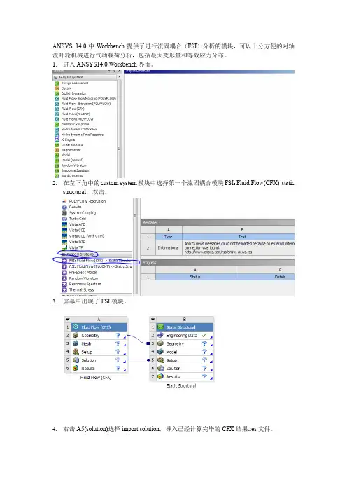
ANSYS 14.0中Workbench提供了进行流固耦合（FSI）分析的模块，可以十分方便的对轴流叶轮机械进行气动载荷分析，包括最大变形量和等效应力分布。

1.进入ANSYS14.0 Workbench界面。

2.在左下角中的custom system模块中选择第一个流固耦合模块FSI：Fluid Flow(CFX)-staticstructural，双击。

3.屏幕中出现了FSI模块。

4.右击A5(solution)选择import solution，导入已经计算完毕的CFX结果.res文件。

5.导入结果后的界面如下图所示。

CFX部分已经完成了计算，所以不需要额外的设置。

6.双击B3（Geometry）进入结构分析的几何单元，初始单位选择meter。

7.导入一个叶片的几何实体，可以选择的几何文件类型很多，x_t、iges等等都可以。

在CFX中，我们通常计算的都是多个转子，多个叶片，但是在分析流固耦合时，只需导入自己关心的那个叶片就可以了。

8.然后点击Generate，就可以看到生成的叶片实体了。

8.关闭Geometry窗口回到Workbench截面，可以看到此时B3(Geometry)后已经变成了绿色的√，说明生成正确。

9.双击B4（model）进入。

可以看到Geometry、coordinate system、connections等项目前面已经是绿色的对号，不需要再进行设置。

10.单击mesh，在左下角的Details of mesh，如图进行设置。

10.右击mesh，选择generate mesh生成网格。

11.生成的叶片网格如图所示。

12.点击static structural ，选择工具栏中的support 下的fixed support，为叶片根部添加约束。

13.选中叶根面，点击左下角中的Apply，完成约束添加。

14.点击上工具栏中units，选择转速单位为RPM.15.如图所示添加转速16.按自己的算例输入转速。

流固耦合定义：它是研究变形固体在流场作用下的各种行为以及固体位形对流场影响这二者相互作用的一门科学。

流固耦合力学的重要特征是两相介质之间的相互作用,变形固体在流体载荷作用下会产生变形或运动。

变形或运动又反过来影响流，从而改变流体载荷的分布和大小，正是这种相互作用将在不同条件下产生形形色色的流固耦合现象。

(一)流固耦合动力学：求解方法与基本理论---张阿漫，戴绍仕●有限元法●边界元法●SPH法与谱单元法●瞬态载荷作用下流固耦合分析方法●小尺度物体的流固耦合振动●水下气泡与边界的耦合效应按耦合机理分两大类：1 耦合作用只发生在两相交界面---界面耦合（场间不相互重叠与渗透），耦合作用通过界面力（包括多相流的相间作用力等）起作用。

它的计算只要满足耦合界面力平衡，界面相容就可以了（其耦合效应是通过在方程中引入两相耦合面边界条件的平衡及协调关系来实现的）。

如气动弹性，水动弹性等。

按照两相间相对运动的大小及相互作用分为三类：(1)流体和固体结构之间有大的相对运动问题"最典型的例子是飞机机翼颤振和悬索桥振荡中存在的气固相互作用问题,一般习惯称为气动弹性力学问题"(2)具有流体有限位移的短期问题"这类问题由引起位形变化的流体中的爆炸或冲击引起"其特点是:我们极其关心的相互作用是在瞬间完成的,总位移是有限的,但流体的压缩性是十分重要的"(3)具有流体有限位移的长期问题"如近海结构对波或地震的响应!噪声振动的响应!充液容器的液固耦合振动!船水响应等都是这类问题的典型例子"对这类问题,主要关心的是耦合系统对外加动力荷载的动态响应"2 两域部分或全部重叠在一起，难以明显的分开，使描述物理现象的方程，特别是本构方程需要针对具体的物理现象来建立，其耦合效应应通过建立与不同单相介质的本构方程等微分方程来体现。

按耦合求解方法分两大类：1 直接耦合求解：直接耦合是在一个求解器中同时求解不同物理场的所有变量，需要针对具体的物理现象来建立本构方程，其耦合效应通过描述问题的微分方程来体现。

例子的来源是Abaqus CLE的官方教程，可是写的太粗线条，我还是搞了两天才做出了这个例子。

其实就是个滚筒洗衣机带着洗衣机里的水一起转的问题。

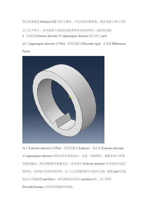
1. 分别为Eulerian domain和Lagrangian domain建立两个part建立Lagrangian domain的Part，类型设置为Discrete rigid，并设置Reference Point。

建立Eulerian domain的Part，类型设置为Eulerian，要注意Eulerian domain 和Lagrangian domain要保证有重叠的部分，这是一种弱耦合，数据在两个区域间抛来抛去，所以网格要有重叠部分。

这导致在Eulerian domain里有的部分是有材料的，有的地方是没有材料的。

为了之后设置材料分布时候方便，要把part实现划出几个辅助的partition。

黄色虚线是在划分partition时，为了指明Extrude/Sweep方向用到的辅助坐标轴。

2. 定义水的材料属性选择状态方程模型EOS中Us-Up，设置声速c0=1483m/s；密度为1000kg/m3；粘度为0.001kg/ms。

并把截面属性赋给Eulerian domain。

3. 把两个Part组装起来4. 新建一个Step-15. 为Eulerian domain和Lagrangian domain划分网格6. 设置接触新建一个Contact Property ，因为不是普通的面和面的接触，水中的任何的一个部分可能在流动区域里的任何一个地方和Lagrangian domain接触，设置Tangential Behavior为Rough，赋给水和洗衣机之间的关系。

新建一个Interaction，把刚才的Contact Property赋给它。

更重要的是设置接触的两个Surface。

其中一个Surface是Lagrangian domain 部分的内侧面，为Geometry类型，另一个Surface是Eulerian domain的全部网格，为Mesh类型。

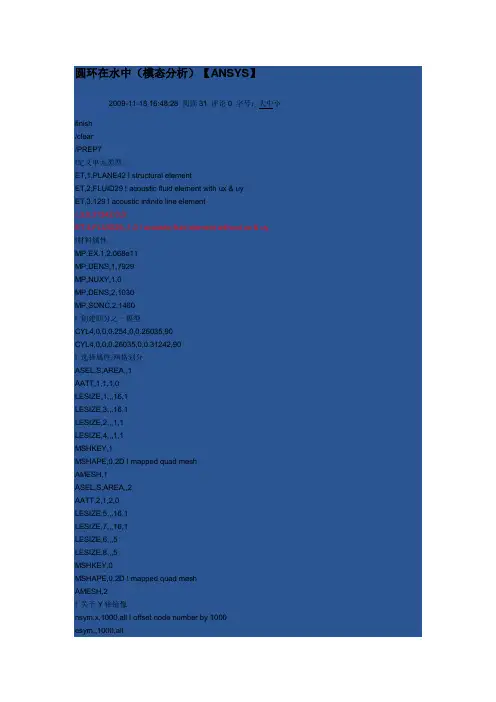
圆环在水中（模态分析）【ANSYS】默认分类2009-11-18 16:48:28 阅读31 评论0 字号：大中小finish/clear/PREP7!定义单元类型ET,1,PLANE42 ! structural elementET,2,FLUID29 ! acoustic fluid element with ux & uyET,3,129 ! acoustic infinite line elementr,3,0.31242,0,0ET,4,FLUID29,,1,0 ! acoustic fluid element without ux & uy!材料属性MP,EX,1,2.068e11MP,DENS,1,7929MP,NUXY,1,0MP,DENS,2,1030MP,SONC,2,1460! 创建四分之一模型CYL4,0,0,0.254,0,0.26035,90CYL4,0,0,0.26035,0,0.31242,90! 选择属性,网格划分ASEL,S,AREA,,1AATT,1,1,1,0LESIZE,1,,,16,1LESIZE,3,,,16,1LESIZE,2,,,1,1LESIZE,4,,,1,1MSHKEY,1MSHAPE,0,2D ! mapped quad meshAMESH,1ASEL,S,AREA,,2AATT,2,1,2,0LESIZE,5,,,16,1LESIZE,7,,,16,1LESIZE,6,,,5LESIZE,8,,,5MSHKEY,0MSHAPE,0,2D ! mapped quad meshAMESH,2! 关于Y轴镜像nsym,x,1000,all ! offset node number by 1000esym,,1000,all! 关于y轴镜像nsym,y,2000,all ! offset node number by 2000esym,,2000,allNUMMRG,ALL ! merge all quantitiesesel,s,type,,1nsle,sesln,s,0 选择附在节点上的单元（0表示单元有一个节点被选中即选中单元）nsle,sesel,inve 反选单元nsle,semodif,all,type,4esel,allnsel,all! 指定无限吸收边界csys,1nsel,s,loc,x,0.31242type,3real,3mat,2esurfesel,allnsel,all! 标识流固交接面nsel,s,loc,x,0.26035esel,s,type,,2sf,all,fsi,1nsel,allesel,allFINISH/soluantype,modalmodopt,damp,10mxpand,10,,,yessolvefinish水箱盛水【ANSYS】默认分类2009-11-18 16:48:38 阅读61 评论0 字号：大中小length=2width=3height=2/prep7et,1,63et,2,30 !选用FLUID30单元，用于流固耦合问题r,1,0.01mp,ex,1,2e11mp,nuxy,1,0.3mp,dens,1,7800mp,dens,2,1000 !定义Acoustics材料来描述流体材料-水mp,sonc,2,1400mp,mu,0,!block,,length,,width,,heightesize,0.5mshkey,1!type,1mat,1real,1asel,u,loc,y,widthamesh,allalls!type,2mat,2vmesh,allfini/soluantype,2modopt,unsym,10 !非对称模态提取方法处理流固耦合问题eqslv,frontmxpand,10,,,1nsel,s,loc,x,nsel,a,loc,x,lengthnsel,r,loc,yd,all,,,,,,ux,uy,uz,nsel,s,loc,y,width,d,all,pres,0allsasel,u,loc,y,width,sfa,all,,fsi !定义流固耦合界面allssolvfini/post1set,firstplnsol,u,sum,2,1finiANSYS 声学计算算例水下圆柱壳体的建模与声学分析使用有限元软件ANSYS进行计算和分析时水下环肋圆柱壳体有限元模型的建立及结构声学分析主要分为以下一些步骤：1.建立壳体的实体模型（包括有圆柱壳体的建立，给圆柱壳体加环肋）；2.圆柱壳体外部流体介质的生成；3.对圆柱壳体和流体介质进行有限元4.设置流固耦合单元，并设置外部声场边界条件；5.在求解器中进行振动模态求解和受激励的谐响应求6.求解结果进行后处理分析。

fluent流固耦合传热算例【原创实用版】目录1.Fluent 流固耦合传热简介2.Fluent 软件的应用范围3.流固耦合传热的算例分析4.Fluent 软件在流固耦合传热中的应用技巧5.总结正文一、Fluent 流固耦合传热简介流固耦合传热是一种复杂的热传递过程，涉及到流体和固体之间的相互作用。

在这种过程中，流体与固体之间的热传递机制和热流动特性都需要考虑。

Fluent 是一款强大的计算流体力学（CFD）软件，可以模拟流固耦合传热过程，为研究人员和工程师提供可靠的解决方案。

二、Fluent 软件的应用范围Fluent 软件广泛应用于各种流体动力学问题的仿真和分析中，包括流固耦合传热问题。

它可以模拟多种流体流动和传热模式，如强制对流、自然对流和湍流等。

同时，Fluent 也可以考虑固体的热传导和热膨胀等特性，为研究者提供全面的热传递分析手段。

三、流固耦合传热的算例分析在 Fluent 中，可以通过设置耦合界面和热流边界条件来模拟流固耦合传热问题。

例如，可以考虑一个流体与固体相接触的系统，通过调整流体和固体的热传导系数、对流换热系数等参数，观察不同条件下的热传递特性。

四、Fluent 软件在流固耦合传热中的应用技巧为了获得准确的仿真结果，需要注意以下几点：1.网格划分：在仿真中，需要对流体和固体部分进行适当的网格划分，以确保计算精度。

2.耦合设置：在设置耦合界面时，需要选择正确的耦合方式，如耦合热流或耦合应力等。

3.边界条件：在设置热流边界条件时，需要考虑流体与固体之间的热交换方式，如对流换热或传导换热等。

4.物质属性：需要正确设置流体和固体的物质属性，如比热容、密度和热传导系数等。

五、总结Fluent 软件在流固耦合传热方面的应用具有广泛的实用性，可以模拟各种复杂的热传递过程。

流固耦合的定义《流固耦合那些事儿》嘿，大家好！今天咱来唠唠“流固耦合”这个听起来有点高大上的玩意儿。

流固耦合嘛，简单说就是流体和固体之间相互影响、相互作用的一种关系。

你想想看哈，水在河里哗哗流，那河边的石头是不是老被水冲来冲去？这就是流体（水）对固体（石头）的作用。

反过来呢，石头要是长得奇形怪状的，也会影响水流的走向吧？这就是固体对流体的影响。

这就是流固耦合在我们生活中常见的例子。

流固耦合就像是一场“拔河比赛”。

流体和固体就像是两队选手，互相拉扯、较劲。

有时候流体力量大，就会把固体冲得摇摇晃晃；有时候固体很顽固，就会让流体拐个弯儿走。

就拿风吹大树来说吧。

风就是那流体，大树就是那固体。

大风呼呼一吹，大树就得跟着晃悠，要是风再大点儿，说不定大树就被吹倒啦！这就是风（流体）和大树（固体）之间的流固耦合。

再比如，咱们盖房子的时候。

房子是固体吧，可要是遇到地震了，那地面晃来晃去的，就跟流体似的。

这时候房子就得承受这种晃动感，要是房子不够结实，那就得遭殃咯！流固耦合的世界啊，充满了各种有趣又奇妙的现象。

有时候让我们头疼，有时候又让我们惊叹。

搞科研的人呢，就喜欢研究这些，想搞清楚流体和固体之间到底是咋互动的。

不过研究流固耦合可不是件容易的事儿啊！就像看一场复杂的“武林争霸赛”，得时刻盯着双方的招式，还得分析出其中的门道。

有时候一个不小心，就可能被复杂的现象给绕晕咯！但这也是它的魅力所在，让人越研究越觉得有意思。

总之呢，流固耦合就是这么个神奇的东西。

它在我们生活中无处不在，影响着我们的方方面面。

无论是大自然中的现象，还是我们人类制造的各种工程，都少不了流固耦合的身影。

所以啊，咱们可得好好认识它、了解它，这样才能更好地和这个奇妙的世界相处嘛！你说是不是这个理儿？。

多孔介质流固耦合模型全文共四篇示例，供读者参考第一篇示例：多孔介质是一种具有孔隙结构的介质，其内部空间可以充满气体或液体。

在工程应用中，多孔介质广泛存在于地下水层、土壤、岩石等领域，其流体运动受到物理和化学环境的复杂影响，因此需要建立多孔介质流固耦合模型来研究其流动特性。

多孔介质流固耦合模型是将多孔介质内部的固相颗粒和流体相耦合起来，通过数学方程描述多孔介质内部的流体流动和固体颗粒的运动规律。

多孔介质流固耦合模型的构建涉及多孔介质内部流动的描述、固相颗粒的运动规律、力学和流体动力学方程的建立等多个方面。

在多孔介质内部的流动描述方面，常用的方法包括达西定律和布里渊方程。

达西定律是描述多孔介质内部流体流动速度与渗透率之间的关系的经典定律，其表示为：\[ v = -K \frac{∇p}{μ} \]v为流速，K为渗透率，p为压力，μ为粘度。

布里渊方程则是描述多孔介质内部流体流动速度随位置变化的变化规律，其表示为：ρ为流体密度，g为重力加速度，z为高度。

达西定律和布里渊方程可以结合使用，建立多孔介质内部流动的数学模型。

固相颗粒的运动规律是多孔介质流固耦合模型的另一个关键方面。

通常情况下，多孔介质内部的固相颗粒会受到流体作用力和固相颗粒之间的相互作用力的影响，其运动规律可以用牛顿第二定律和达西定律描述。

牛顿第二定律表示为：\[ F = ma \]F为作用力，m为质量，a为加速度。

达西定律描述了固相颗粒受到的流体作用力与流速之间的关系。

通过以上分析，我们可以看出，多孔介质流固耦合模型是描述多孔介质内部流动和固相颗粒运动的重要数学模型，其建立需要考虑多个方面的因素。

在实际工程应用中，多孔介质流固耦合模型可以用于研究地下水流动、土壤固结、岩石力学等问题，为工程设计和科学研究提供重要的参考依据。

希望通过本文的介绍，读者能够对多孔介质流固耦合模型有更深入的了解，并在实际应用中取得更好的研究成果。

第二篇示例：多孔介质是一种具有孔隙结构的材料，它可以允许流体通过或在其中存储流体。

流固耦合分析（FSI）流固耦合分析（FSI）是涉及流体和固体之间相互作用的问题研究，其理论包括了几个主要方面：流体力学、固体力学、耦合边界条件、求解器等。

以下是流固耦合分析的详细理论讲解，带有相关公式和尽量详细的说明。

一、流体力学1. 守恒定律质量守恒定律：$$ \frac{\partial \rho}{\partial t} + \nabla \cdot (\rho \mathbf{u}) = 0 $$动量守恒定律：$$ \rho \frac{\partial \mathbf{u}}{\partial t} + \rho (\mathbf{u} \cdot \nabla) \mathbf{u} = \nabla \cdot \tau + \mathbf{f} $$其中，$\rho$是流体密度，$\mathbf{u}$是流体速度，$\tau$是应力张量，$\mathbf{f}$是体力。

2. 纳维-斯托克斯方程$$ \rho \frac{\partial \mathbf{u}}{\partial t} + \rho (\mathbf{u} \cdot \nabla) \mathbf{u} = \nabla \cdot (-p\mathbf{I} + \tau) + \mathbf{f} $$其中，$p$是静压力，$\mathbf{I}$是单位张量。

3. 边界条件（1）速度边界条件：$\mathbf{u} = \mathbf{u}_b$，其中$\mathbf{u}_b$是边界上的速度。

（2）压力边界条件：$p = p_b$，其中$p_b$是边界上的压力。

4. 流体力学求解器常用的流体力学求解器有OpenFOAM、ANSYS Fluent等。

二、固体力学1. 力学基本方程$$ \tau = \sigma\cdot \mathbf{n} $$其中，$\tau$是表面上的接触力，$\sigma$是固体的应力张量，$\mathbf{n}$是表面的单位法向量。

流固耦合问题流固耦合问题是一种复杂的物理问题，它涉及到流体和固体之间的相互作用。

这种问题常常出现在工程设计和生物医学领域中，比如船舶设计、飞机设计、药物输送等。

本文将分步骤阐述流固耦合问题的相关知识。

第一步：理解流固耦合问题的概念流固耦合问题是指涉及到流动和固体材料之间相互作用的物理问题。

它通常发生在可变形固体与流体之间的边界面上，例如在弹性材料的表面或开放溶液表面。

由于流体和固体的相互作用，物体的形状和运动状态会发生变化。

这种变化可能会对流体运动状态产生影响，从而改变流体的速度和压力分布。

第二步：了解流固耦合问题的类别流固耦合问题可分为两类，一种是静态耦合，另一种是动态耦合。

静态耦合是指在瞬间时间内，固体形变速度远小于流体速度的情况下发生的耦合作用。

动态耦合是指在一段时间内，固体形变和流体运动是相互影响的耦合作用。

在生物医学领域中，由于心脏的收缩和血液的流动是相互影响的动态耦合，因此对这种耦合的研究极为重要。

第三步：分析流固耦合问题的数学模型流固耦合问题的数学模型通常由连续性、动量守恒和边值条件三个方程组成。

其中，连续性方程描述了流体的质量守恒，动量守恒方程描述了流体的运动状态，边值条件则用于描述固体表面的物理特性。

根据实际问题需要，可以采用不同的数值解法对模型进行求解，例如有限元法、有限体积法和边界元法等。

第四步：应用流固耦合问题的实际案例流固耦合问题在工程设计和生物医学领域中都有广泛的应用。

例如，在飞机设计中，需要考虑飞机表面的气流对于飞机结构的影响；在生物医学领域中，需要研究血流对心脏、大脑和肝脏等器官的作用。

此外，在船舶设计、岩土工程和涂料涂装等领域中也需要考虑流固耦合问题。

总之，流固耦合问题是一个非常重要的物理问题，在工程设计和生物医学领域有着广泛的应用。

深入研究流固耦合问题的数学模型和求解方法，能够为相关领域的进一步发展提供重要的理论和实践支持。

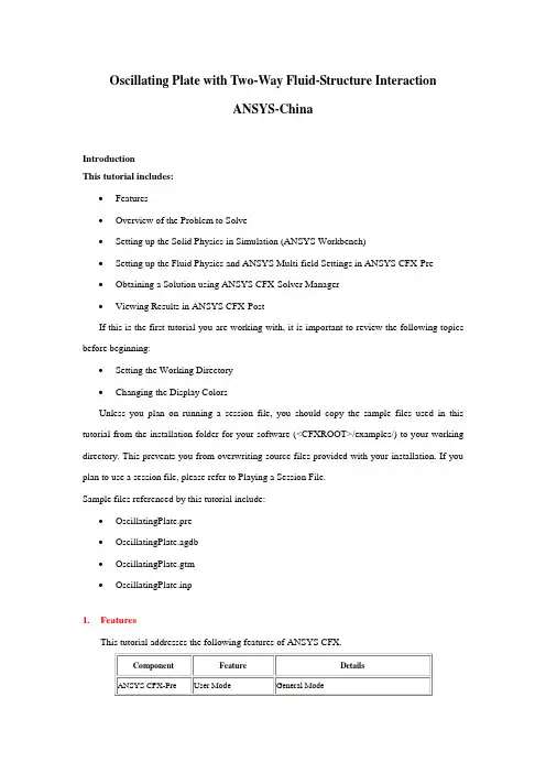
Oscillating Plate with Two-Way Fluid-Structure InteractionANSYS-ChinaIntroductionThis tutorial includes:∙Features∙Overview of the Problem to Solve∙Setting up the Solid Physics in Simulation (ANSYS Workbench)∙Setting up the Fluid Physics and ANSYS Multi-field Settings in ANSYS CFX-Pre∙Obtaining a Solution using ANSYS CFX-Solver Manager∙Viewing Results in ANSYS CFX-PostIf this is the first tutorial you are working with, it is important to review the following topics before beginning:∙Setting the Working Directory∙Changing the Display ColorsUnless you plan on running a session file, you should copy the sample files used in this tutorial from the installation folder for your software (<CFXROOT>/examples/) to your working directory. This prevents you from overwriting source files provided with your installation. If you plan to use a session file, please refer to Playing a Session File.Sample files referenced by this tutorial include:∙OscillatingPlate.pre∙OscillatingPlate.agdb∙OscillatingPlate.gtm∙OscillatingPlate.inp1.FeaturesThis tutorial addresses the following features of ANSYS CFX.In this tutorial you will learn about:∙Moving mesh∙Fluid-solid interaction (including modeling solid deformation using ANSYS)∙Running an ANSYS Multi-field (MFX) simulation∙Post-processing two results files simultaneously.2.Overview of the Problem to SolveThis tutorial uses a simple oscillating plate example to demonstrate how to set up and run a simulation involving two-way Fluid-Structure Interaction, where the fluid physics is solved in ANSYS CFX and the solid physics is solved in the FEA package ANSYS. Coupling between the two solvers is required throughout the solution to model the interaction between fluid and solid as time progresses, and the framework for the coupling is provided by the ANSYS Multi-field solver, using the MFX setup.The geometry consists of a 2D closed cavity. A thin plate is anchored to the bottom of the cavity as shown below:An initial pressure of 100 Pa is applied to one side of the thin plate for 0.5 seconds in order to distort it. Once this pressure is released, the plate oscillates backwards and forwards as it attempts to regain its equilibrium (vertical) position. The surrounding fluid damps the oscillations, which therefore have an amplitude that decreases in time. The CFX Solver calculates how the fluid responds to the motion of the plate, and the ANSYS Solver calculates how the plate deforms as a result of both the initial applied pressure and the pressure resulting from the presence of the fluid. Coupling between the two solvers is required since the solid deformation affects the fluid solution, and the fluid solution affects the solid deformation.The tutorial describes the setup and execution of the calculation including the setup of the solid physics in Simulation (within ANSYS Workbench) and the setup of the fluid physics and ANSYS Multi-field settings in ANSYS CFX-Pre. If you do not have ANSYS Workbench, then you can use the provided ANSYS input file to avoid the need for Simulation.3.Setting up the Solid Physics in Simulation (ANSYS Workbench)This section describes the step-by-step definition of the solid physics in Simulation within ANSYS Workbench that will result in the creation of an ANSYS input file OscillatingPlate.inp. If you prefer, you can instead use the provided OscillatingPlate.inp file and continue from Setting up the Fluid Physics and ANSYS Multi-field Settings in ANSYS CFX-Pre.Creating a New Simulation1.If required, launch ANSYS Workbench.2.Click Empty Project. The Project page appears displaying an unsaved project.3.Select File > Save or click Save button.4.If required, set the path location to a different folder. The default location is your workingdirectory. However, if you have a specific folder that you want to use to store files created during this tutorial, change the path.5.Under File name, type OscillatingPlate.6.Click Save.7.Under Link to Geometry File on the left hand task bar click Browse. Select the providedfile OscillatingPlate.agdb and click Open.8.Make sure that OscillatingPlate.agdb is highlighted and click New simulation from theleft-hand taskbar.Creating the Solid Material1.When Simulation opens, expand Geometry in the project tree at the left hand side of theSimulation window.2.Select Solid, and in the Details view below, select Material.e the arrow that appears next to the material name Structural Steel to select NewMaterial.4.When the Engineering Data window opens, right-click New Material from the tree viewand rename it to Plate.5.Enter 2.5e06 for Young's Modulus, 0.35 for Poisson's Ratio and 2550 for Density.Note that the other properties are not used for this simulation, and that the units for these values are implied by the global units in Simulation.6.Click the Simulation tab near the top of the Workbench window to return to thesimulation.Basic Analysis SettingsThe ANSYS Multi-field simulation is a transient mechanical analysis, with a timestep of 0.1 s and a time duration of 5 s.1.Select New Analysis > Flexible Dynamic from the toolbar.2.Select Analysis Settings from the tree view and in the Details view below, set Auto TimeStepping to Off.3.Set Time Step to 0.1.4.Under Tabular Data at the bottom right of the window, set End Time to5.0 for theSteps = 1 setting.Inserting LoadsLoads are applied to an FEA analysis as the equivalent of boundary conditions in ANSYS CFX. In this section, you will set a fixed support, a fluid-solid interface, and a pressure load. Fixed SupportThe fixed support is required to hold the bottom of the thin plate in place.1.Right-click Flexible Dynamic in the tree and select Insert> Fixed Support from theshortcut menu.2.Rotate the geometry using the Rotate button so that the bottom (low-y) face of thesolid is visible, then select Face and click the low-y face.That face should be highlighted to indicate selection.3.Ensure Fixed Support is selected in the Outline view, then, in the Details view, selectGeometry and click 1 Face to make the Apply button appear (if necessary). Click Apply to set the fixed support.Fluid-Solid InterfaceIt is necessary to define the region in the solid that defines the interface between the fluid in CFX and the solid in ANSYS. Data is exchanged across this interface during the execution of the simulation.1.Right-click Flexible Dynamic in the tree and select Insert > Fluid Solid Interface fromthe shortcut menu.ing the same face-selection procedure described earlier, select the three faces of thegeometry that form the interface between the solid and the fluid (low-x, high-y and high-x faces) by holding down <Ctrl> to select multiple faces. Note that this load is automatically given an interface number of 1.Pressure LoadThe pressure load provides the initial additional pressure of 100 [Pa] for the first 0.5 seconds of the simulation. It is defined using a step function.1.Right-click Flexible Dynamic in the tree and select Insert > Pressure from the shortcutmenu.2.Select the low-x face for Geometry.3.In the Details view, select Magnitude, and using the arrow that appears, select Tabular(Time).4.Under Tabular Data, set a pressure of 100 in the table row corresponding to a time of 0.Note: The units for time and pressure in this table are the global units of [s]and [Pa], respectively.5.You now need to add two new rows to the table. This can be done by typing the new timeand pressure data into the empty row at the bottom of the table, and Simulation will automatically re-order the table in order of time value. Enter a pressure of 100 for a time value of 0.499, and a pressure of 0 for a time value of 0.5.This gives a step function for pressure that can be seen in the chart to the left of the table. Writing the ANSYS Input FileThe Simulation settings are now complete. An ANSYS Multi-field run cannot be launched from within Simulation, so the Solve buttons cannot be used to obtain a solution.1.Instead, highlight Solution in the tree, select Tools> Write ANSYS Input File andchoose to write the solution setup to the file OscillatingPlate.inp.2.The mesh is automatically generated as part of this process. If you want to examine it,select Mesh from the tree.3.Save the Simulation database, use the tab near the top of the Workbench window to returnto the Oscillating Plate [Project] tab, and save the project itself.4.Setting up the Fluid Physics and ANSYS Multi-field Settings in ANSYS CFX-PreThis section describes the step-by-step definition of the flow physics and ANSYS Multi-field settings in ANSYS CFX-Pre.Playing a Session FileIf you want to skip past these instructions and to have ANSYS CFX-Pre set up the simulation automatically, you can select Session > Play Tutorial from the menu in ANSYS CFX-Pre, then run the session file: OscillatingPlate.pre. After you have played the session file as described in earlier tutorials under Playing the Session File and Starting ANSYS CFX-Solver Manager, proceed to Obtaining a Solution using ANSYS CFX-Solver Manager.Creating a New Simulation1.Start ANSYS CFX-Pre.2.Select File > New Simulation.3.Select General and click OK.4.Select File > Save Simulation As.5.Under File name, type OscillatingPlate.6.Click Save.Importing the Mesh1.Right-click Mesh and select Import Mesh.2.Select the provided mesh file, OscillatingPlate.gtm and click Open.Note：The file that was just created in Simulation, OscillatingPlate.inp, will be used as an input file for the ANSYS Solver.Setting the Simulation TypeA transient ANSYS Multi-field run executes as a series of timesteps. The Simulation Type tab is used both to enable an ANSYS Multi-field run and to specify the time-related settings for it (in the External Solver Coupling settings). The ANSYS input file is read by ANSYS CFX-Pre so that it knows which Fluid Solid Interfaces are available.Once the timesteps and time duration are specified for the ANSYS Multi-field run (coupling run), ANSYS CFX automatically picks up these settings and it is not possible to set the timestep and time duration independently. Hence the only option available for Time Duration is Coupling Time Duration, and similarly for the related settings Time Step and Initial Time.1. ClickSimulation Type .2. Apply the following settings3. Click OK .Note ：You may see a physics validation message related to the difference in the units used in ANSYS CFX-Pre and the units contained within the ANSYS input file. While it is important to review the units used in any simulation, you should be aware that, in this specific case, the message is not crucial as it is related to temperature units and there is no heat transfer in this case. Therefore, this specific tutorial will not be affected by the physics message. Creating the FluidA custom fluid is created with user-specified properties. 1. Click Material.2. Set the name of the new material to Fluid.3. Apply the following settings4.Click OK.Creating the DomainIn order to allow the ANSYS Solver to communicate mesh displacements to the CFX Solver, mesh motion must be activated in CFX.1.Right click Simulation in the Outline tree view and ensure that Automatic DefaultDomain is selected. A domain named Default Domain should now appear under the Simulation branch.2.Double click Default Domain and apply the following settings3.Click OK.Creating the Boundary ConditionsIn addition to the symmetry conditions, another type of boundary condition corresponding with the interaction between the solid and the fluid is required in this tutorial.Fluid Solid External BoundaryThe interface between ANSYS and CFX is defined as an external boundary in CFX that has its mesh displacement being defined by the ANSYS Multi-field coupling process.When an ANSYS Multi-field specification is being made in ANSYS CFX-Pre, it is necessary to provide the name and number of the matching Fluid Solid Interface that was created in Simulation. Since the interface number in Simulation was 1, the name in question is FSIN_1. (If the interface number had been 2, then the name would have been FSIN_2, and so on.)On this boundary, CFX will send ANSYS the forces on the interface, and ANSYS will send back the total mesh displacement it calculates given the forces passed from CFX and the other defined loads.1.Create a new boundary condition named Interface.2.Apply the following settings3.Click OK.Symmetry BoundariesSince a 2D representation of the flow field is being modeled (using a 3D mesh with one element thickness in the Z direction) symmetry boundaries will be created on the low and high Z 2D regions of the mesh.1.Create a new boundary condition named Sym1.2.Apply the following settings3.Click OK.4.Create a new boundary condition named Sym2.5.Apply the following settings6.Click OK.Setting Initial ValuesSince a transient simulation is being modeled, initial values are required for all variables.1. ClickGlobal Initialization. 2. Apply the following settings:3. Click OK .Setting Solver ControlVarious ANSYS Multi-field settings are contained under Solver Control under the External Coupling tab. Most of these settings do not need to be changed for this simulation.Within each timestep, a series of “coupling” or “stagger” iterations are performed to ensure that CFX, ANSYS and the data exchanged between the two solvers are all consistent. Within each stagger iteration, ANSYS and CFX both run once each, but which one runs first is a user-specifiable setting. In general, it is slightly more efficient to choose the solver that drives the simulation to run first. In this case, the simulation is being driven by the initial pressure applied in ANSYS, so ANSYS is set to solve before CFX within each stagger iteration.1. Click Solver Control .2. Apply the following settings:3.Click OK.Setting Output ControlThis step sets up transient results files to be written at set intervals.1.Click Output Control .2.On the Trn Results tab, create a new transient result with the default name.3.Apply the following settings to Transient Results 1:4.Click the Monitor tab.5.Select Monitor Options.6.Under Monitor Points and Expressions:7.Click Add new item and accept the default name.8.Set Option to Cartesian Coordinates.9.Set Output Variables List to Total Mesh Displacement X.10.Set Cartesian Coordinates to [0, 1, 0].11.Click OK.Writing the Solver (.def) File1.Click Write Solver File .2.If the Physics Validation Summary dialog box appears, click Yes to proceed.3.Apply the following settings4.Ensure Start Solver Manager is selected and click Save.5.If you are notified the file already exists, click Overwrite.6.This file is provided in the tutorial directory and will exist in your working folder if youhave copied it there.7.Quit ANSYS CFX-Pre, saving the simulation (.cfx) file at your discretion.5.Obtaining a Solution using ANSYS CFX-Solver ManagerThe execution of an ANSYS Multi-field simulation requires both the CFX and ANSYS solvers to be running and communicating with each other. ANSYS CFX-Solver Manager can be used to launch both solvers and to monitor the output from both.1.Ensure the Define Run dialog box is displayed.There is a new MultiField tab which contains settings specific for an ANSYS Multi-field simulation.2.On the MultiField tab, check that the ANSYS input file location is correct (the location isrecorded in the definition file but may need to be changed if you have moved files around).3.On UNIX systems, you may need to manually specify where the ANSYS installation is ifit is not in the default location. In this case, you must provide the path to the v110/ansys directory.4.Click Start Run.The run begins by some initial processing of the ANSYS Multi-field input which results in the creation of a file containing the necessary multi-field commands for ANSYS, and then the ANSYS Solver is started. The CFX Solver is then started in such a way that it knows how to communicate with the ANSYS Solver.After the run is under way, two new plots appear in ANSYS CFX-Solver Manager:ANSYS Field Solver (Structural) This plot is produced only when the solid physics is set to use large displacements or when other non-linear analyses are performed. It shows convergence of the ANSYS Solver. Full details of the quantities are described in the ANSYS user documentation. In general, the CRIT quantities are the convergence criteria for each relevant variable, and the L2 quantities represent the L2 Norm of the relevant variable. For convergence, the L2 Norm should be below the criteria. The x-axis of the plot is the cumulative iteration number for ANSYS, which does not correspond to either timesteps or stagger iterations. Several ANSYS iterations will beperformed for each timestep, depending on how quickly ANSYS converges. You will usually see a somewhat “spiky” plot, as each quantity will be unconverged at the start of each time step, and then convergence will improve.ANSYS Interface Loads (Structural)This plot shows the convergence for each quantity that is part of the data exchanged between the CFX and ANSYS Solvers. In this case, four lines appear, corresponding to two force components (FX and FY) and two displacement components (UX and UY). Since the analysis is 2D, FZ and UZ are not exchanged. Each quantity is converged when the plot shows a negative value. The x-axis of the plot corresponds to the cumulative number of stagger iterations (coupling iterations) and there are several of these for every timestep. Again, a spiky plot is expected as the quantities will not be converged at the start of a timestep.The ANSYS out file is displayed in ANSYS CFX-Solver Manager as an extra tab. Similar to the CFX out file, this is a text file recording output from ANSYS as the solution progresses.1.Click the User Points tab and watch how the top of the plate displaces as the solutiondevelops.2.When the solvers have finished and ANSYS CFX-Solver Manager puts up a dialog boxto tell you this, click Yes to post-process the results.3.If using Standalone Mode, quit ANSYS CFX-Solver Manager.6.Viewing Results in ANSYS CFX-PostFor an ANSYS Multi-field run, both the CFX and ANSYS results files will be opened up in ANSYS CFX-Post by default if ANSYS CFX-Post is started from a finished run in ANSYS CFX-Solver Manager.Plotting Results on the SolidWhen ANSYS CFX-Post reads an ANSYS results file, all the ANSYS variables are available to plot on the solid, including stresses and strains. The mesh regions available for plots by default are limited to the full boundary of the solid, plus certain named regions which are automatically created when particular types of load are added in Simulation. For example, any Fluid Solid Interface will have a corresponding mesh region with a name such as FSIN 1. In this case, there is also a named region corresponding to the location of the fixed support, but in general pressure loads do not result in a named region.You can add extra mesh regions for plotting by creating named selections in Simulation - see the Simulation product documentation for more details. Note that the named selection must have a name which contains only English letters, numbers and underscores for the named mesh region to be successfully created.Note that when ANSYS CFX-Post loads an ANSYS results file, the true global range for each variable is not automatically calculated, as this would add a substantial amount of time onto how long it takes to load such a file (you can turn on this calculation using Edit > Options and using the Pre-calculate variable global ranges setting under CFX-Post> Files). When the global range is first used for plotting a variable, it is calculated as the range within the current timestep. As subsequent timesteps are loaded into ANSYS CFX-Post, the Global Range is extended each time variable values are found outside the previous Global Range.1.Turn on the visibility of Boundary ANSYS (under ANSYS > Domain ANSYS).2.Right-click a blank area in the viewer and select Predefined Camera > View Towards-Z. Zoom into the plate to see it clearly.3.Apply the following settings to Boundary ANSYS:4.Click Apply.5.Select Tools> Timestep Selector from the task bar to open the Timestep Selectordialog box. Notice that a separate list of timesteps is available for each results file loaded, although for this case the lists are the same. By default, Sync Cases is set to By Time Value which means that each time you change the timestep for one results file, ANSYS CFX-Post will automatically load the results corresponding to the same time value for all other results files.6.Set Match to Nearest Available.7.Change to a time value of 1 [s] and click Apply.The corresponding transient results are loaded and you can see the mesh move in both the CFX and ANSYS regions.1.Clear the visibility check box of Boundary ANSYS.2.Create a contour plot, set Locations to Boundary ANSYS and Sym2, and set Variable toTotal Mesh Displacement. Click Apply.ing the timestep selector, load time value 1.1 [s] (which is where the maximum totalmesh displacement occurs).This verifies that the contours of Total Mesh Displacement are continuous through both the ANSYS and CFX regions.Many FSI cases will have only relatively small mesh displacements, which can make visualization of the mesh displacement difficult. ANSYS CFX-Post allows you to visually magnify the mesh deformation for ease of viewing such displacements. Although it is not strictly necessary for this case, which has mesh displacements which are easily visible unmagnified, this is illustrated by the next few instructions.ing the timestep selector, load time value 0.1 [s] (which has a much smaller meshdisplacement than the currently loaded timestep).2.Place the mouse over somewhere in the viewer where the background color is showing.Right-click and select Deformation > Auto. Notice that the mesh displacements are now exaggerated. The Auto setting is calculated to make the largest mesh displacement a fixed percentage of the domain size.3.To return the deformations to their true scale, right-click and select Deformation > TrueScale.Creating an Animationing the Timestep Selector dialog box, ensure the time value of 0.1 [s] is loaded.2.Clear the visibility check box of Contour 1.3.Turn on the visibility of Sym2.4.Apply the following settings to Sym2.5.Click Apply.6.Create a vector plot, set Locations to Sym1 and leave Variable set to Velocity. SetColor to be Constant and choose black. Click Apply.7.Select the visibility check box of Boundary ANSYS, and set Color to a constant blue.8.Click Animation .The Animation dialog box appears.9.Select Keyframe Animation.10.In the Animation dialog box:a.Click New to create KeyframeNo1.b.Highlight KeyframeNo1, then change # of Frames to 48.c.Load the last timestep (50) using the timestep selector.d.Click New to create KeyframeNo2.The # of Frames parameter has no effect for the last keyframe, so leave it at thedefault value.e.Select Save MPEG.f.Click Browse next to the MPEG file data box to set a path and file name forthe MPEG file.If the file path is not given, the file will be saved in the directory from whichANSYS CFX-Post was launched.g.Click Save.The MPEG file name (including path) will be set, but the MPEG will not becreated yet.h.Frame 1 is not loaded (The loaded frame is shown in the middle of theAnimation dialog box, beside F:). Click To Beginning to load it then waita few seconds for the frame to load.i.Click Play the animation .The MPEG will be created as the animation proceeds. This will be slow, since atimestep must be loaded and objects must be created for each frame. To view theMPEG file, you need to use a viewer that supports the MPEG format.11.When you have finished, exit ANSYS CFX-Post.12.。

CAE联盟论坛精品讲座系列基于MpCCI的Abaqus和Fluent流固耦合案例主讲人：mafuyin CAE联盟论坛总监摘要：通过MpCCI流固耦合接口程序，对某薄壁管道流动中的传热过程进行了Abaqus和Fluent相结合的流固耦合仿真分析。

信息介绍了从建模、设置到求解计算和后处理的全过程，对相关研究人员具有参考意义。

1 分析模型用三维建模软件solidworks建立了一个管径为1m的弯管，结构尺寸如图1a所示，管的结构如图1b所示，流体的模型如图1c所示。

值得注意的是，由于拓扑特征的原因，这样的管壁模型无法通过对圆环扫略直接生成，而需先通过对大圆的扫略生成实心的模型(类似于流体模型)，然后进行抽壳得到管壁的模型。

用同样的方法对大圆半径减去管壁厚度的圆进行扫略得到流体模型。

a. 尺寸关系b. 管壁结构c. 流体模型图1. 几何模型示意图图2. 流固耦合传热分析模型示意图内壁面(耦合面)速度入口v=6m/s; T in=600K外壁面压力出口P=0Pa；T out=300K由于管壁结构和流体的热学行为不同，传热系数等都不一样，所以属于典型的流固耦合传热问题，热学模型如图2所示。

即管的一端为流体速度入口，一端为压力出口，给定流体外壁面一个初始温度600K，流体入口速度为6m/s，温度为600K，出口相对大气压力为0Pa，出口温度为300K。

需要求解流体和管壁的温度场分布情况。

2 流体模型将图1c的流体模型以Step格式导入Fluent软件通常使用的前处理器Gambit中，如图3a所示。

设置求解器为，然后划分体网格，网格尺寸为100mm，类型为六面体单元，一共生成4895个体单元，网格如图3b所示。

a. 导入Gambit软件中的流体模型b. 流场的网格模型图3. 流体模型及网格示意图进行网格划分后，需定义边界条件，在Gambit软件中先分别定义速度入口(VELOCITY_INLET)、压力出口(PRESSURE_OUTLET)和壁面(Wall)三组边界条件，具体参数设置在Fluent软件中进行。

第五章 轴流泵的流固耦合5-1 流固耦合概论流固耦合问题一般分为两类，一类是流‐固单向耦合，一类是流‐固双向耦合。

单向耦合应用于流场对固体作用后，固体变形不大，即流场的边界形貌改变很小，不影响流场分布的，可以使用流固单向耦合。

先计算出流场分布，然后将其中的关键参数作为载荷加载到固体结构上。

典型应用比如小型飞机按刚性体设计的机翼，机翼有明显的应力受载，但是形变很小，对绕流不产生影响。

当固体结构变形比较大，导致流场的边界形貌发生改变后，流场分布会有明显变化时，单向耦合显然是不合适的，因此需要考虑固体变形对流场的影响，即双向耦合。

比如大型客机的机翼，上下跳动量可以达到5 米，以及一切机翼的气动弹性问题，都是因为两者相互影响产生的。

因此在解决这类问题时，需要进行流固双向耦合计算。

下面简单介绍其理论基础。

连续流体介质运动是由经典力学和动力学控制的，在固定产考坐标系下，它们可以被表达为质量、动量守恒形式:()0v tρρ∂+∇⋅=∂ (1) ()B v vv f tρρτ∂+∇⋅-=∂ (2) 式中，ρ为流体密度；v 为速度向量；Bf 流体介质的体力向量；τ为应力张量；在旋转的参考坐标系下，控制方程变为： ()0r v v tρρ∂+∇⋅=∂ （3） (-)+B r r c v v v f f tρρτ∂+∇⋅=∂ （4） 形式和固定坐标系下基本相同，只是速度变成了相对速度，另外就是增加了附加力项c f 。

固体有限元动力控制方程为：[]{}[]{}{}...[]{}M u C u K u F ++= （5）式中，[]M ，[]C ，[]K 分别是质量矩阵，阻尼矩阵以及刚度矩阵，{}F 为载荷矩阵。

流固耦合遵循最基本的守恒原则，所以在流固耦合交界面处，应满足流体与固体应力、位移、热流量、温度等变量的相等或守恒，即满足如下四方程：f f s s n n ττ⋅=⋅ (6)f s d d = (7)f s q q = (8)f s T T = (9)5-2 单向流固耦合思路分析：轴流泵的单向流固耦合仅仅考虑流场对结构的影响，并不考虑结构变形对流场的影响，所以其数据的传递是单向的，流场和结构的分开计算，完成流场计算之后将其作为结构的边界条件加载到结构域上。

流固耦合计算实例Oscillating Plate with Two-Way Fluid-Structure InteractionANSYS-ChinaIntroductionThis tutorial includes:Features* Overview of the Problem to SolveSetti ng up the Solid Physics in Simulatio n (ANSYS Workbe nch)Setti ng up the Fluid Physics and ANSYS Multi-field Setti ngs in ANSYS CFX-PreObta ining a Solution using ANSYS CFX-Solver Ma nagerViewi ng Results in ANSYS CFX-PostIf this is the first tutorial you are working with, it is important to review the following topics before begi nning:* Sett ing the Worki ng Directory* Cha nging the Display ColorsUni ess you pla n on running a sessi on file, you should copy the sample files used in this tutorial from the in stallati on folder for your software (/examples/) to your work ing directory. This preve nts you from overwriti ng source files provided with your in stallatio n. If you pla n to use a sessi on file, please refer to Play ing a Sessi on File.Sample files refere need by this tutorial in clude:* Oscillati ngPlate.pre* Oscillati ngPlate.agdb* Oscillat in gPlate.gtm* Oscillati ngPlate.i np1. FeaturesIn this tutorial you will lear n about:Moving mesh* Fluid-solid in teract ion (in cludi ng modeli ng solid deformati on using ANSYS)* Running an ANSYS Multi-field (MFX) simulatio n* Post-process ing two results files simulta neously.2. Overview of the Problem to SolveThis tutorial uses a simple oscillat ing plate example to dem on strate how to set up and run a simulation involving two-way Fluid-Structure Interaction, where the fluid physics is solved in ANSYS CFX and the solid physics is solved in the FEA package ANSYS. Coupling between the two solvers is required throughout the soluti on to model the in teract ion betwee n fluid and solid as time progresses, and the framework for the coupli ng is provided by the ANSYS Multi-field solver, using the MFX setup.The geometry con sists of a 2D closed cavity. A thin plate is an chored to the bottom of the cavity as show n below:An in itial pressure of 100 Pa is applied to one side of the thin plate for 0.5 sec onds in order to distort it. Once this pressure is released, the plate oscillates backwards and forwards as it attempts to regain its equilibrium (vertical) position. The surrounding fluid damps the oscillations, which therefore have an amplitude that decreases in time. The CFX Solver calculates how the fluid resp onds to the moti on of the plate, and the ANSYS Solver calculates how the plate deforms as a result of both the in itial applied pressure and the pressure result ing from the prese nee of the fluid. Coupli ng betwee n the two solvers isrequired si nee the solid deformati on affects the fluid soluti on, and the fluid solution affects the solid deformation.The tutorial describes the setup and execution of the calculation including the setup of the solid physics in Simulati on (withi n ANSYS Workbe nch) and the setup of the fluid physics and ANSYS Multi-field sett ings in ANSYS CFX-Pre. If you do n ot have ANSYS Workbe nch, the n you can use the provided ANSYS in put file to avoid the n eed for Simulatio n.3. Setting up the Solid Physics in Simulation (ANSYS Workbench)This secti on describes the step-by-step defi niti on of the solid physics in Simulati on with in ANSYS Workbe nch that will result in the creation of an ANSYS in put file Oscillati ngPlate.i np. If you prefer, you can in stead use the provided Oscillati ngPlate.i np file and continue from Sett ing up the Fluid Physics and ANSYS Multi-field Setti ngs in ANSYS CFX-Pre.Creating a New Simulatio n1. If required, lau nch ANSYS Workbe nch.2. Click Empty Project. The Project page appears displaying an unsaved project.3. Select File > Save or click Save butt on.4. If required, set the path location to a different folder. The default location is your workingdirectory. However, if you have a specific folder that you want to use to store files createdduring this tutorial, change the path.5. Un der File name, type Oscillat in gPlate.6. Click Save.7. Under Link to Geometry File on the left hand task bar clickBrowse. Select the providedfile OscillatingPlate.agdb and click Open.8. Make sure that OscillatingPlate.agdb is highlighted and click New simulation from the left-ha nd taskbar.Creati ng the Solid Material1. When Simulatio n ope ns, expa nd Geometry in the project tree at the left hand side of theSimulatio n win dow.2. Select Solid, and in the Details view below, select Material .3. Use the arrow that appears next to the material name Structural Steel to select NewMaterial .4. When the Engineering Data window ope ns, right-click New Material from the tree viewand ren ame it to Plate.乱i i i ii-.i1 ir - 11 j j| -|^i y <="">Ffe UrWi T^i IH AW - - - 丙5. Enter 2.5e06 for Young's Modulus , 0.35 for Poisson's Ratio and 2550 for Density.Note that the other properties are not used for this simulati on, and that the un its for thesevalues are implied by the global un its in Simulati on.6. Click the Simulation tab near the top of the Workbench window to return to the simulatio n. Basic An alysis Sett ings The ANSYS Multi-field simulation is a transient mechanical analysis, with a timestep of 0.1 s anda time duration of 5 s.1. Select New Analysis > Flexible Dynamic from the toolbar.2. Select An alysis Setti ngs from the tree view and in theDetails view below, set Auto TimeStepping to Off.3. Set Time Step to 0.1.1 t Hwt&riw 期* MalffQ冠SbiUcHMl 5诟* 工L on vwMani {IpAgridiri AM 匕■曲亡■■4. Under Tabular Data at the bottom right of the window, set End Time to5.0 for the Steps =1 sett in g.Inserting LoadsLoads are applied to an FEA an alysis as the equivale nt of boun dary con diti ons in ANSYS CFX. In this sect ion, you will set a fixed support, a fluid-solid in terface, and a pressure load.Fixed SupportThe fixed support is required to hold the bottom of the thin plate in place.1. Right-click Flexible Dynamic in the tree and select Insert > Fixed Support from the shortcutmenu.2. Rotate the geometry using the Rotate butt on so that the bottom (low-y) face of thesolid is visible, then select Face 囲and click the low-y face.That face should be highlighted to in dicate selecti on.3. Ensure Fixed Support is selected in the Outline view, then, in the Details view, selectGeometry and click 1 Face to make the Apply butt on appear (if n ecessary). Click Apply to set the fixed support.Fluid-Solid InterfaceIt is n ecessary to defi ne the regi on in the solid that defi nes the in terface betwee n the fluid in CFX and the solid in ANSYS. Data is excha nged across this in terface duri ng the executi on of the simulatio n.1. Right-click Flexible Dynamic in the tree and select Insert > Fluid Solid Interface fromthe shortcut menu.2. Using the same face-selection procedure described earlier, select the three faces of thegeometry that form the in terface betwee n the solid and the fluid (low-x, high-y and high-xfaces) by holding down to select multiple faces. Note that this load is automaticallygive n an in terface nu mber of 1.Pressure LoadThe pressure load provides the in itial additi onal pressure of 100 [Pa] for the first 0.5 sec onds of the simulati on .It is defi ned using a step function.1. Right-click Flexible Dyn amic in the tree and select Insert > Pressure from the shortcutmenu.2. Select the low-x face for Geometry.3. In the Details view, select Magnitude , and using the arrow that appears, select Tabular(Time).4. Under Tabular Data , set a pressure of 100 in the table row corresponding to a time of 0.Note: The units for time and pressure in this table are the global units of [s] and [Pa], respectively.5. You now n eed to add two new rows to the table. This canbe done by typi ng the new timeand pressure data into the empty row at the bottom of the table, and Simulation willautomatically re-order the table in order of time value. Enter a pressure of 100 for a timevalue of 0.499, and a pressure of 0 for a time value of 0.5.This gives a step function for pressure that can be see n in the chart to the left of the table. Writi ng the ANSYS In put File The Simulation settings are now complete. An ANSYS Multi-field run cannot be launched from with in Simulati on, so the Solve butt ons cannot be used to obta in a soluti on.1. In stead, highlight Solution in the tree, select T ools > Write ANSYS Input File and chooseto write the solution setup to the file OscillatingPlate.inp.2. The mesh is automatically gen erated as part of this process. If you want to exam ine it,select Mesh from the tree.3. Save the Simulation database, use the tab near the top of the Workbench window to returnto the Oscillating Plate [Project] tab, and save the project itself.4. Setting up the Fluid Physics and ANSYS Multi-field Settings in ANSYS CFX-PreThis section describes the step-by-step definition of the flow physics and ANSYS Multi-field settings in ANSYS CFX-Pre.Playing a Session FileIf you want to skip past these instructions and to have ANSYS CFX-Pre set up the simulation automatically, you can select Session> Play Tutorial from the menu in ANSYS CFX-Pre, then runthe session file: OscillatingPlate.pre. After you have played the session file as described in earlier tutorials under Playing the Session File and Starting ANSYS CFX-Solver Manager, proceed to Obtaining a Solution using ANSYS CFX-Solver Manager.Creating a New Simulation1. Start ANSYS CFX-Pre.2. Select File > New Simulation .3. Select General and click OK.4. Select File > Save Simulation As.5. Under File name, type OscillatingPlate.6. Click Save.Importing the Mesh1. Right-click Mesh and select Import Mesh .2. Select the provided mesh file, OscillatingPlate.gtm and click Open.Note：The file that was just created in Simulation, OscillatingPlate.inp, will be used as an input file for the ANSYS Solver.Setting the Simulation TypeA transient ANSYS Multi-field run executes as a series of timesteps. The Simulation Type tab is used both to enable an ANSYS Multi-field run and to specify the time-related settings for it (in the External Solver Coupling settings). The ANSYS input file is read by ANSYS CFX-Pre so that it knows which Fluid Solid Interfaces are available.Once the timesteps and time duration are specified for the ANSYS Multi-field run (coupling run), ANSYS CFX automatically picks up these settings and it is not possible to set the timestep and time duration independently. Hence the only option available for Time Duration is Coupling Time Duration, andsimilarly for the related settings Time Step and Initial Time.。

fluent流固耦合传热算例fluent流固耦合传热算例是针对流体和固体之间热量传递的一种数值模拟方法。

在工程领域中，流固耦合传热问题广泛存在于换热器、散热器、核电站等领域，对于优化设计、提高传热效率以及解决实际工程问题具有重要意义。

一、流固耦合传热概念介绍流固耦合传热是指在流体与固体之间由于温度差引起的热量传递过程。

在这种传热方式中，流体和固体的温度场、速度场以及压力场之间存在相互影响的关系。

流固耦合传热问题可以分为内部耦合和外部耦合两种类型。

内部耦合是指流体和固体内部的热量传递过程，而外部耦合是指流体和固体之间的热量交换。

二、流固耦合传热算例背景及意义本文以某实际工程为背景，通过fluent软件对流固耦合传热问题进行数值模拟。

旨在揭示流体与固体之间热量传递的规律，为实际工程提供参考依据。

通过分析算例，可以优化传热装置设计，提高传热效率，降低能耗，从而降低生产成本。

三、算例具体内容与分析本算例采用fluent软件进行数值模拟，考虑流体在固体内部的流动与热量传递。

模拟过程中，流体与固体的温度、速度、压力等参数随时间和空间的变化关系。

通过计算得到流体与固体之间的热量交换，从而分析传热过程的性能。

四、结果讨论与启示通过对流固耦合传热算例的分析，得到以下结论：1.在流固耦合传热过程中，流体的温度分布和速度分布对固体表面的热量传递有显著影响。

2.固体内部的温度分布存在一定的规律，可通过优化固体材料、改变流体流动方式等方法提高传热效果。

3.流固耦合传热问题具有较强的非线性特点，需要采用数值模拟方法进行深入研究。

本算例为实际工程提供了有益的参考，启示我们在设计传热装置时，要充分考虑流体与固体之间的相互作用，从而实现高效、节能的目标。

综上所述，fluent流固耦合传热算例对于揭示流体与固体之间热量传递规律具有重要的实际意义。

第十一章流固耦合分析LS-DYNA除了具有强大的结构动力分析模块外，还具有强大的流体与固体相互耦合的功能，广泛应用于各种爆炸（水下、空中、建筑物和土壤中）、气囊展开、体积成型，罐内液体晃动等分析中。

下面具体讨论怎样应用LS-DYNA进行流固耦合分析及应该注意的一些问题，也希望通过本章的学习对LS-DYNA流固耦合分析方法有深入的了解和掌握。

11.1 Lagrangian、Eulerisn和ALE算法在LS-DYNA中三维单元有三种基本的算法：Lagrangian、Eulerisn和ALE（任意拉格朗日欧拉算法）算法，是由关键字*SECTION_SOLID中的ELFORM控制的:从上面可知ELFORM的取值不一样导致单元算法的不一样，可用于流固耦合分析的单元公式如下（不包括1）：1 = 常应力实体单元（纯粹的Lagrangian算法）5 = 中心单点积分的ALE算法（单元内为单一材料）6 = 中心单点积分的Eulerisn单元（单元内为单一材料）7 = 中心单点积分的环境Eulerisn单元（用于Eulerisn计算的进出口边界）11 = 中心单点积分的ALE多物质单元（一个单元内可以包含多种物质）12 = 中心单点积分的带空白材料的单物质ALE单元149150Lagrangian 、Eulerisn 和ALE 算法的区别算法的区别：：LS-DYNA 程序具有Lagrange 、Euler 和ALE 算法，Lagrange 算法的单元网格附着在材料上，随着材料的流动而产生单元网格的变形。

但是在结构变形过于巨大时，有可能使有限元网格造成严重畸变，引起数值计算的困难，甚至程序终止运算。

ALE 算法和Euler 算法可以克服单元严重畸变引起的数值计算困难，并实现流体-固体耦合的动态分析。

ALE 算法先执行一个或几个Lagrange 时步计算，此时单元网格随材料流动而产生变形，然后执行ALE 时步计算：（1）保持变形后的物体边界条件，对内部单元进行重分网格，网格的拓扑关系保持不变，称为Smooth Step ；（2）将变形网格中的单元变量（密度、能量、应力张量等）和节点速度矢量输运到重分后的新网格中，称为Advection Step 。