《高级微观经济学Advanced Microeconomics》课件PPT-l
- 格式:ppt
- 大小:561.00 KB
- 文档页数:23
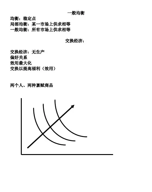
一般均衡均衡:稳定点局部均衡:某一市场上供求相等一般均衡:所有市场上供求相等交换经济:交换经济:无生产偏好关系效用最大化交换以提高福利(效用)两个人、两种禀赋商品Edgeworth 图 禀赋点为e假设自主交换能够实现帕累托改进,达到更优的配置点x对消费者1,其所偏好e 的区域为红色区域,最终的配置点必须在这一区域内,否那么,他拒绝交换或抵制这一配置。
对消费者2,其所偏好e 的区域为蓝色区域,最终的配置点必须在这一区域内,否那么,他拒绝交换或抵制这一配置。
因此,最终的配置点必须在重叠的区域中——凸透镜区域内和边上。
在这一区域里,双方或至少一方的福利能够提高。
11ee设交换后形成的配置点'x 在凸透镜内部,双方福利都得到改善,同时各有一条无差异曲线交于此点。
双方进一步通过交换改善彼此福利。
对消费者1,其所偏好'x 的区域为红色区域,最终的配置点必须在这一区域内,否那么,他拒绝交换或抵制这一配置。
对消费者2,其所偏好'x 的区域为蓝色区域,最终的配置点必须在这一区域内,否那么,他拒绝交换或抵制这一配置。
因此,最终的配置点必须在重叠的区域中——凸透镜区域内和边上。
在这一区域里,双方或至少一方的福利能够提高。
11ee'x交换过程持续下去,凸透镜越来越小,最终变为一个点:两条无差异曲线的切点:x 。
此时,双方进一步交换会使某一方福利下降。
所以,双方的交换一旦达到了切点位置,就不会有交换发生。
实现了帕累托最优。
在凸透镜内部和边上,这样的点有无数多个,最终的配置究竟是哪一个点,我们并不知道,或者说,我们不知道决定最终的帕累托效率点的位置的因素是什么。
结论只是:帕累托效率点位于凸透镜边上或内部的某个切点位置上。
11eexEdgeworth图中,所有的无差异曲线的切点的连线构成契约线,帕累托效率点是凸透镜与契约线交集中的点。
2 11eex当禀赋点落在契约线上时,即为帕累托效率点,无交换发生。


Advanced Microeconomics Topic 3: Consumer DemandPrimary Readings: DL – Chapter 5; JR - Chapter 3; Varian, Chapters 7-9.3.1 Marshallian Demand FunctionsLet X be the consumer's consumption set and assume that the X = R m +. For a given price vector p of commodities and the level of income y , the consumer tries to solve the following problem:max u (x )subject to p ⋅x = y x ∈ X• The function x (p , y ) that solves the above problem is called the consumer's demand function .• It is also referred as the Marshallian demand function . Other commonly known namesinclude Walrasian demand correspondence/function , ordinary demand functions , market demand functions , and money income demands .• The binding property of the budget constraint at the optimal solution, i.e., p ⋅x = y , is theWalras’ Law .• It is easy to see that x (p , y ) is homogeneous of degree 0 in p and y .Examples:(1) Cobb-Douglas Utility Function:.,...,1,0 ,)(1m i x x u i mi i i =>=∏=ααFrom the example in the last lecture, the Marshallian demand functions are:.ii i p yx αα=where∑==mi i 1αα.(2) CES Utility Functions: )10( )(),(/12121<≠+=ρρρρx x x x uThen the Marshallian demands are:,),( ;),(2112221111rr r r r r p p yp y x p p y p y x +=+=--p p where r = ρ/(ρ -1). And the corresponding indirect utility function is given byrr r p p y y v /121)(),(-+=pLet us derive these results. Note that the indirect utility function is the result of the utility maximization problem:yx p x p x x x x =++2211/121, subject to )(max 21ρρρDefine the Lagrangian function:)()(),,(2211/12121y x p x p x x x x L -+-+=λλρρρThe FOCs are:00)(0)(22112121)/1(2121111)/1(211=-+=∂∂=-+=∂∂=-+=∂∂----y x p x p Lp x x x x L p x x x x L λλλρρρρρρρρ Eliminating λ, we get⎪⎩⎪⎨⎧+=⎪⎪⎭⎫⎝⎛=-2211)1/(12121x p x p y p p x x ρ So the Marshallian demand functions are:rr r rrr p p yp y x x p p yp y x x 211222211111),(),(+==+==--p pwith r = ρ/(ρ-1). So the corresponding indirect utility function is given by:r r r p p y y x y x u y v /12121)()),(),,((),(-+==p p p3.2 Optimality Conditions for Co nsumer’s ProblemFirst-Order ConditionsThe Lagrangian for the utility maximization problem can be written asL = u (x ) - λ( p ⋅x - y ).Then the first-order conditions for an interior solution are:yu i p x u i i =⋅=∇∀=∂∂x p p x x λλ)( i.e. ;)( (1)Rewriting the first set of conditions in (1) leads to,,k j p p MU MU MRS kj kj kj ≠==which is a direct generalization of the tangency condition for two-commodity case.Sufficiency of First-Order ConditionsProposition : Suppose that u (x ) is continuous and quasiconcave on R m +, and that (p , y ) > 0. If u if differentiable at x*, and (x*, λ*) > 0 solves (1), then x* solve the consumer's utility maximization problem at prices p and income y .Proof . We will use the following fact without a proof:• For all x , x ' ≥ 0 such that u (x') ≥ u (x ), if u is quasiconcave and differentiable at x , then∇u (x )(x' - x ) ≥ 0.Now suppose that ∇u (x*) exists and (x*, λ*) > 0 solves (1). Then,∇u (x*) = λ*p , p ⋅x* = y .If x* is not utility-maximizing, then must exist some x 0 ≥ 0 such thatu (x 0) > u (x*) and p ⋅x 0 ≤ y .Since u is continuous and y > 0, the above inequalities implies thatu (t x 0) > u (x*) and p ⋅(t x 0) < yfor some t ∈ [0, 1] close enough to one. Letting x' = t x 0, we then have∇u (x*)(x' - x ) = (λ*p )⋅( x' - x ) = λ*( p ⋅x' - p ⋅x ) < λ*(y - y ) = 0,which contradicts to the fact presented at the beginning of the proof since u (x 1) > u (x*).Remark• Note that the requirement that (x*, λ*) > 0 means that the result is true only forinterior solutions.Roy's IdentityNote that the indirect utility function is defined as the "value function" of the utility maximization problem. Therefore, we can use the Envelope Theorem to quickly derive the famous Roy's identity.Proposition (Roy's Identity?): If the indirect utility function v (p , y ) is differentiable at (p 0, y 0) and assume that ∂v (p 0, y 0)/ ∂y ≠ 0, then.,...,1 ,),(),(),(000000m i yy v p y v y x ii =∂∂∂∂-=p p pProof . Let x * = x (p , y ) and λ* be the optimal solution associated with the Lagrangian function:L = u (x ) - λ( p ⋅x - y ).First applying the Envelope Theorem, to evaluate ∂v (p 0, y 0)/ ∂p i gives.**)*,(),(*i ii x p L p y v λλ-=∂∂=∂∂x p But it is clear that λ* = ∂v (p , y )/ ∂y , which immediately leads to the Roy's identity.Exercise• Verify the Roy's identity for CES utility function.Inverse Demand FunctionsSometimes, it is convenient to express price vector in terms of the quantity demanded, which leads to the so-called inverse demand functions .• the inverse demand function may not always exist. But the following conditions willguarantee the existence of p (x ):• u is continuous, strictly monotonic and strictly quasiconcave. (In fact, these conditionswill imply that the Marshallian demand functions are uniquely defined.)Exercise (Duality of Indirect and Direct Demand Functions):(1) Show that for y = 1 the inverse demand function p = p (x ) is given by:.,...,1 ,)()()(1m i x x u x u p m j j jii =∂∂∂∂=∑=x x x(Consult JR, pp.79-80.)(2) Show that for y = 1, the (direct) demand function x = x (p, 1) satisfies.,...,1 ,)1,()1,()1,(1m i p p v p v x m j j j ii =∂∂∂∂=∑=p p p(Hint: Use Roy’s identity and the homogeneity of degree zero of the indirect uti lityfunction.)3.3 Hicksian Demand FunctionsRecall that the expenditure function e (p , u ) is the minimum-value function of the following optimization problem:,)( s.t. min ),(u u u e m≥⋅=+∈x x p p R x for all p > 0 and all attainable utility levels.It is clear that e (p , u ) is well-defined because for p ∈ R m ++, x ∈ R m +, p ⋅x ≥ 0.If the utility function u is continuous and strictly quasiconcave, then the solution to the above problem is unique, so we can denote the solution as the function x h (p , u ) ≥ 0. By definition, it follows thate (p , u ) = p ⋅x h (p , u ).• x h (p , u ) is called the compensated demand functions , also commonly known as Hicksiandemand functions , named after John Hicks when he first discussed this type of demand functions in 1939.Remarks1. The reason that they are called "compensated " demand function is that we mustimpose an artificial income adjustment when the price of one good is changing while the utility level is assumed to be fixed.2. It is important to understand that, in contrast with the Marshallian demands, theHicksian demands are not directly observable.As usual, it should be no longer a surprise that there is a close link between the expenditure function and the Hicksian demands, as summarized in the following result, which is again a direct application of the Envelope Theorem..Proposition (Shephard's Lemma for Consumer): If e (p , u ) is differentiable in p at (p 0, u 0) with p 0 > 0, then,.,...,1 ,),(),(000m i p u e u x ih i=∂∂=p pExample: CES Utility Functions)10( )(),(/12121<≠+=ρρρρx x x x uLet us now derive the Hicksian demands and the corresponding expenditure function.min {p 1x 1 + p 2x 2} subject to)(/121u x x =+ρρρThe Lagrangian function is))((),,(/121221121u x x x p x p x x L -+-+=ρρρλλThen the FOCs are:0)(0)((0)((/121121/12122111/12111=+-=∂∂=+-=∂∂=+-=∂∂----ρρρρρρρρρρρλλλx x u L x x x p x L x x x p x L Eliminating λ, we getρρρρ/121)1/(12121)(x x u p p x x +=⎪⎪⎭⎫ ⎝⎛=- From these, it is easy to derive the Hicksian demand functions given by:121)/1(212111)/1(211)(),()(),(----+=+=r r r r h r r r r h pp p u u x p p p u u x p pwhere r = ρ/(ρ-1). And the expenditure function is.)(),(),(),(/1212211rr r h h p p u u x p u x p u e +=+=p p pAlternatively, since we know that the indirect utility function is given by:,)(),(/121rr r p p y y v -+=p3.4 Recall that (last the indirect utility function v (p (a) e (p , v (b) v (p , eFurthermore, we solutions ofboth optimization the following interesting identities between Marshallian demands and Hicksian demands:x (p , y ) = x h (p , v (p , y )) x h (p , u ) = x (p , e (p , u ))which hold for all values of p , y and u .The second identity leads to a classic differentiation relation between Hicksian demands and Marshallian demands, known as Slutsky equation.Proposition (Slutsky Equation): If the Marshallian and Hicksian demands are all well-defined and continuously differentiable, then for p > 0, x > 0,),,(),(),(),(y x yy x p u x p y x j i j h i j i p p p p ⋅∂∂-∂∂=∂∂where u = v (p , y ).Proof . It follows easily from taking derivative and applying Shephard's Lemma.Substitution and Income Effects• The significance of Slutsky equation is that it decomposes the change caused by a pricechange into two effects: a substitution effect and an income effect .• The substitution effect is the change in compensated demand due to the change inrelative prices, which is the first item in Slutsky equation.• The income effect is the change in demand due to the effective change in incomecaused by the price change, which is the second item in Slutsky equation. • The substitution effect is unobservable, while the income effect is observable.Question: From the above diagram (also know as Hicksian decomposition ), can you see crossing property between a Marshallian demand function and the corresponding Hicksian demand? (Hint: there are two general cases.)Slutsky MatrixThe substitution effect between good i and good j is measured byj i p u x s jh i ij ,,),(∀∂∂=pSo the Slutsky matrix or the substitution matrix is the m ⨯m matrix of the substitution items:⎥⎥⎦⎤⎢⎢⎣⎡∂∂==j h i ij p u x s ),(][p SThe following result summarizes the basic properties of the Slutsky matrix.Proposition (Substitution Properties). The Slutsky matrix S is symmetric and negative semidefinite.Proof . By Shephard’s Lemma (for consumer), we know thatji ihj i j j i j h i ij s p u x p p u e p p u e p u x s =∂∂=∂∂∂=∂∂∂=∂∂=),(),(),(),(22p p p pHence S is symmetric. It is evident that S is the Hessian matrix of the expenditure function e (p , u ).Since we know that e (p , u ) is concave, so its Hessian matrix must be negative semidefinite.Since the second-order own partial derivatives of a concave function are always nonpositive, this implies that s ii ≤ 0, i.e.,i p u x s ih i ii ∀≤∂∂=,0),(pwhich indicates the intuitive property of a demand function: as its own price increases, the quantity demanded will decrease. You are reminded that this is a general property for Hicksian demands.For the Marshallian demands, note that by Slutsky equation,).,(),(),(),(y x yy x p u x p y x i i i h i i i p p p p ⋅∂∂-∂∂=∂∂Then for a small change in p i , we will have the following:.),(),(),(),(i i i i i h i i i i i p y x yy x p p u x p p y x x ∆⋅∂∂-∆∂∂=∆∂∂≈∆p p p pThe first item, capturing the own price effect of the Hicksian demands, is of course nonpositive.The sign of the second item depends on the nature of the good:• Normal good : ∂x i (p , y )/ ∂y > 0.• This leads to a normal Marshallian demand function: it is decreasing in its ownprice.• Inferior good : ∂x i (p , y )/ ∂y < 0.• When the substitution effect still dominates the income effect, the resultingMarshallian demand is also decreasing in its own price.• When the substitution effect is dominated by the income effect, it will lead to aGiffen good, that is, its demand function is an increasing function of its own price.Because of Slutsky equation, the Slutsky matrix (i.e., the substitution matrix) also has the following form that is in terms of Marshallian demand functions.⎥⎥⎦⎤⎢⎢⎣⎡∂∂+∂∂=⎥⎥⎦⎤⎢⎢⎣⎡∂∂==),(),(),(),(][y x y y x p y x p u x s j i j i j h i ij p p p p SWe will get back to the above Slutsky matrix in the next lecture when we discuss the integrability problem .3.5. The Elasticity Relations for Marshallian Demand FunctionsDefinition . Let x (p , y ) be the consumer’s Marshallian demand functions. Define.),(,),(),(,),(),(yy x p s y x p p y x y x yy y x i i i i jj i ij i i i p p p p p =∂∂=∂∂=εηThen1. ηi is called the income elasticity of demand for good i .2. ε ij is called the price elasticity of the demand for good i with respect to a price change ingood j . ε ii is the own-price elasticity of the demand for good i . For i ≠ j , ε ij is the cross-price elasticity .3. s i is called the income share spent on good i .The following result summarizes some important relationships among the income shares, income elasticities and the price elasticities.Proposition . Let x (p , y ) be the consumer’s Marshallian demand functions. Then1. Engel aggregation :.11=∑=mi ii s η2. Cournot aggregation :.,...,1 ,1m j s s j mi iji =-=∑=εProof . Both identities are derived from the Walras’ Law, namely, the fact that the budget is tight or balanced:y = p ⋅x (p , y ) for all p and y . (A)To prove Engel aggregation, we differentiate both sides of (A) w.r.t. y :∑∑∑====∂∂=∂∂=m i mi i i ii i i mi i i s y x yy y x y y x p y y x p 111,),(),(),(),(1ηp p p pas required.To prove Cournot aggregation, we differentiate both sides of (A) w.r.t. p j :.),(),(),(),(),(01∑∑=≠∂∂=-⇒∂∂++∂∂=mi j i i j jj jj ji j i ip y x p y x p y x p y x p y x p p p p p pMultiplying both sides by p j /y leads to∑∑∑====-⇒∂∂=∂∂=-mi iji j mi i jj i i i mi j j i i j j s s y x p p y x y y x p p p y x y p yy x p 111),(),(),(),(),(εp p p p pas required too.3.6 Hicks ’ Composite Commodity TheoremAny group of goods & services with no change in relative prices between themselves may be treated as a single composite commodity, with the price of any one of the group used as the price of the composite good and the quantity of the composite good defined as the aggregate value of the whole group divided by this price. Important use in applied economic analysis.Additional ReferencesAfriat, S. (1967) "The Construction of Utility Functions from Expenditure Data," International Economic Review, 8, 67-77.Arrow, K. J. (1951, 1963) Social Choice and Individual Values. 1st Ed., Yale University Press, New Haven, 1951; 2nd Ed., John Wiley & Sons, New York, 1963.Becker, G. S. (1962) "Irrational Behavior and Economic Theory," Journal of Political Economy, 70, 1-13.Cook, P. (1972) "A One-line Proof of the Slutsky Equation," American Economic Review, 42, 139. Deaton, A. and J. Muellbauer (1980) Economics and Consumer Behavior. Cambridge University Press, Cambridge.Debreu, G. (1959) Theory of Value. John Wiley & Sons, New York.Debreu, G. (1960) "Topological Methods in Cardinal Utility Theory," in Mathematical Methods in the Social Sciences, ed. K. J. Arrow and M. D. Intriligator, North Holland, Amsterdam. Diewert, W. E. (1982) "Duality Approaches to Microeconomic Theory," Chapter 12 in Handbook of Mathematical Economics, ed. K. J. Arrow and M. D. Intriligator, North Holland, Amsterdam.Gorman, T. (1953) “Community Preference Fields,” Econometrica, 21, 63-80.Hicks, J. (1946) V alue and Capital. Clarendon Press, Oxford, England.Katzner, D.W. (1970) Static Demand Theory. MacMillan, New York.Marshall, A. (1920) Principle of Economics, 8th Ed. MacMillan, London.McKenzie, L. (1957) “Demand Theory Without a Utility In dex," Review of Economic Studies, 24, 183-189.Pollak, R. (1969) "Conditional Demand Functions and Consumption Theory," Quarterly Journal of Economics, 83, 60-78.Roy, R. (1942) De l'utilite. Hermann, Paris.Roy, R. (1947) "La distribution de revenu entre les divers biens," Econometrica, 15, 205-225. Samuelson, P. A. (1938) "A Note on the Pure Theory of Consumer's Behavior," Econometrica, 5, 61-71, 353-354.Samuelson, P. (1947) Foundations of Economic Analysis. Harvard University Press, Cambridge, Massachusetts.Sen, (1970) Collective Choice and Social Welfare. Holden Day, San Francisco.Stigler, G. (1950) "Development of Utility Theory," Journal of Political Economy, 59, parts 1 & 2, pp. 307-327, 373-396.Varian, H. R. (1992) Microeconomic Analysis. Third Edition. W.W. Norton & Company, New York. (Chapters 7, 8 and 9)Wold, H. and L. Jureen (1953) Demand Analysis. John Wiley & Sons, New York.11。

Chapter1:Key conceptsFebruary19,20131IntroductionEconomics is the study of choice under scarcity.Typically,consumers want more goods and services than they can afford to buy.Similarly,businesses face constraints in terms what funds and resources that they can ernments and countries also face the same type of problem:a government might want to address a large number of social problems,but they have limited resources with which to do so.Economics is about understanding how a party deals with the fact that when they use their resources to pursue one option,they cannot use those resources to do something else.And so,a consumer may have to choose between a new pair of shoes or a textbook,afirm may have to choose between developing a new product or launching a marketing campaign, and the government may have to choose between improving education or targeting crime.To understand these issues,economics has developed a set of tools that can be used to analyze these problems.This book provides an introduction to those tools.They can be used to help understand economic problems wherever they arise,be it businesses understanding the markets they compete in,or governments trying to develop social policy,or families trying to manage their households.These tools are not meant to capture everything that is occurring in any given situation.Rather,they are designed to simplify(or to model)a complicated and potentially messy real-world issue into a tractable form that can provide valuable insights.Given that resources are limited,the key questions that an economy needs to‘decide’are:(a)what to produce;(b)how to produce it;and(c)who should get what is made.In modern economies,the answers to these questions are largely determined by the market –that is,by the interaction of sellers and buyers in the market.1Sometimes,however, the government also helps determine the answer to these questions,by regulating or intervening in the market.Consequently,our focus in this microeconomics text will be on the study of individuals(consumers,firms,and governments)and their interaction in markets.This chapter provides a few key concepts that underpin the analysis in the rest of the book,as well as economics analysis in general.1By‘market’,we simply mean a place where buyers and sellers of a particular good or service meet, such as a traditional bazaar or an online trading site.12Scarcity and opportunity costAs noted above,it is usually the case that resources are limited,so that not all wants can be met.We call this situation scarcity.Scarcity also means that individuals,businesses and societies face tradeoffs;by choos-ing one thing,a person must give up or miss out on another thing.For example,if a consumer uses their money to buy product X,they cannot then use that same money to buy something else.2We use the concept of opportunity cost to measure that tradeoff. Thus,the opportunity cost of any choice is the value of the best forgone alternative. In the example above,if the consumer buys product X,and the next best thing they could have done is buy product Y,the opportunity cost of buying X is forgoing Y.Individuals also face opportunity costs in terms of their time–that is,if a person spends his time doing one thing,he cannot also spend that time doing another.Example.Suppose Andrew prefers to spend his Saturday afternoon walk-ing.The next best thing that he could have done is to sleep,and his thirdbest choice is to go swimming.Therefore,if Andrew goes for a walk,the op-portunity cost of going for a walk is not sleeping,as this is his best foregoneopportunity.The option of swimming is not relevant here because it is notthe next best opportunity.Opportunity costs include both explicit costs and implicit costs.Explicit costs are costs that involve direct payment(or,in other words,would be considered as costs by an accountant).Implicit costs are opportunities that are forgone,but do not involve an explicit cost.3Example.Suppose Stephen decides to go to university,and his next bestoption is to work at a construction site and earn$80K over the year.Theexplicit costs are those that Stephen must directly pay to go to university,such as student fees,the cost of textbooks,and so on.The implicit costsare the opportunities that Stephen must forgo–that is,working at theconstruction site and earning$80K.It is important to note that opportunity cost only includes costs that could change if a different decision were made.Opportunity cost does not include sunk(or unrecoverable) costs.Sunk costs are costs that have been incurred and cannot be recovered no matter what.For example,if Katrien spends the weekend reading an accounting textbook, no matter what she does(such as whether or not she decides to continue studying accounting),she cannot get that time back.Similarly,if a business spent$100K on an advertising campaign last year,regardless of what they decide to do this year,that money(and effort)cannot be recovered.2It is common to hear people refer to the‘economics’of a particular thing.This colloquial statement really means that,given the limited resource available,a choice had to be made and something(possibly worthwhile)could not be done.3Sometimes,economists distinguish between‘economic costs’and‘accounting costs’.Economic costs is just another term for opportunity costs,and therefore includes explicit and implicit costs. Accounting costs refers to explicit costs only.23Marginal analysisTypically,we assume that economic agents are rational and act to maximize their benefits from their economic transactions.4For example,consumers seek to maximize their benefits from consumption andfirms seek to maximize their profits from production. One way that economic agents can solve this maximization problem is by considering the additional benefit or additional cost of any action.This sort of analysis is referred to as marginal analysis and it is a recurring theme both in this book and economics generally.For instance,consider a consumer faced with the decision of whether to buy one more unit of a particular good.That consumer might consider the extra benefit he derives from buying that extra unit;this is referred to as the marginal benefit of that extra unit of the good.The consumer might also consider the additional cost of buying one more unit;this is referred to as the marginal cost of purchasing another unit,which is typically the price of the good.In making theirfinal decision,the consumer will weigh the marginal benefit against the marginal cost of buying that extra unit.For example, if a consumer is considering buying another cup of coffee,and the marginal benefit is$5 and the marginal cost is$3,the consumer will be better offby buying the extra coffee.Each of the marginal terms noted above,and many others,will be discussed at length throughout the book.What is crucial to note is that the term‘marginal’simply means means additional or extra.That is,we interested to see what happens if we increase things(such as the number of coffees bought)by a small amount.4Ceteris paribusThe notion of ceteris paribus is also an important foundation of economic analysis.As noted,because the real world is often complicated and messy,it is often necessary to simplify real-world situations into tractable economic models,in order to better analyze them.Thus,in order to determine the effect of a particular thing,economists tend to examine the impact of one change at a time,holding everything else constant.This is often called ceteris paribus,which roughly means‘other things equal’.For instance,suppose we are interested in how a change in price will affect the quantity demanded of a good.However,in reality,demand for a good can be affected by a number of other factors,such as changes in the tastes or income of consumers,or the availability or price of substitute goods.Therefore,in order to isolate the effect of price upon quantity demanded,we need hold everything else constant.This is not to deny that in the real world multiple changes can occur at a time–they often do.Rather, to fully understand the relationship between price and demand,it is essential to isolate that relationship from other events that might also be occurring.For example,afirm 4We are not suggesting that,in the real word,consumers are always fully rational or thatfirms do not sometimes have other objectives.Rather,we adopt this simplifying assumption because it allows us to analyze the behaviour of economic agents in markets.Such analysis will be fairly accurate,provided that on average individual consumers andfirms act more or less in their own interest.3might be interested in the effect of advertising on demand for its product.To understand the impact of advertising,it is crucial to remove other factors that could affect demand, otherwise advertising could be attributed too much(or too little)influence,which could lead to poor decision-making by thefirm regarding its next advertising campaign.5Correlation and causationAnother factor to keep in mind is the difference between correlation and causation. Correlation refers to a situation in which two or more things are observed to move together(or against each other).On the other hand,causation refers to a situation where changes in one thing brings about or causes change in another thing.To make statements about causation requires an economic theory about how the world works, rather than just observing a statistical relationship between several variables.Sometimes,when we observe correlation between two variables,A and B,it is because one causes the other.Sometimes,it is because a third factor causes changes in A and B(like a rising tide causing two boats to rise in their moorings).Sometimes,there is no connection between the two variables and it is just by chance that we observed the change in both variables at the same time.Without a theory about how a change in one variable affects the other,it is not possible to say which is the case.4。