斯托克,沃森计量经济学第七章实证练习stata

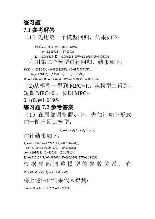
练习题7.1参考解答（1）先用第一个模型回归，结果如下：22216.4269 1.008106 t=(-6.619723) (67.0592)R 0.996455 R 0.996233 DW=1.366654 F=4496.936PCE PDI =-+==利用第二个模型进行回归，结果如下：122233.27360.9823820.037158 t=(-5.120436) (6.970817) (0.257997)R 0.996542 R 0.996048 DW=1.570195 F=2017.064t t t PCE PDI PCE -=-++==（2)从模型一得到MPC=1.；从模型二得到，短期MPC=0.，长期MPC= 0.+(0.)=1.01954练习题7.2参考答案（1）在局部调整假定下，先估计如下形式的一阶自回归模型：*1*1*0*tt ttu Y X Y +++=-ββα估计结果如下：122ˆ15.104030.6292730.271676 se=(4.72945) (0.097819) (0.114858)t= (-3.193613) (6.433031) (2.365315)R =0.987125 R =0.985695 F=690.0561 DW=1.518595t t t Y X Y -=-++根据局部调整模型的参数关系，有****11 ttu u αδαβδββδδ===-=将上述估计结果代入得到： *1110.2716760.728324δβ=-=-=*20.738064ααδ==-*0.864001ββδ==故局部调整模型估计结果为： *ˆ20.7380640.864001ttYX =-+ 经济意义解释：该地区销售额每增加1亿元，未来预期最佳新增固定资产投资为0.亿元。

运用德宾h 检验一阶自相关：(121(1 1.34022d h =-=-⨯=在显著性水平05.0=α上，查标准正态分布表得临界值21.96h α=，由于21.3402 1.96h h α=<=，则接收原假设0=ρ，说明自回归模型不存在一阶自相关。

计量经济学斯托克沃森第三版答案1、盈余公积是企业从（）中提取的公积金。

[单选题] *A.税后净利润(正确答案)B.营业利润C.利润总额D.税前利润2、企业在转销已经确认无法支付的应付账款时，应贷记的会计科目是（）。

[单选题] *A.其他业务收入B.营业外收入(正确答案)C.盈余公积D.资本公积3、企业因解除与职工的劳动关系给予职工补偿而发生的职工薪酬，应借记的会计科目是（）。

[单选题] *A.管理费用(正确答案)B.计入存货成本或劳务成本C.营业外支出D.计入销售费用4、由投资者投资转入的无形资产，应按合同或协议约定的价值，借记“无形资产”科目，按其在注册资本所占的份额，贷记“实收资本”科目，按其差额记入（）科目。

[单选题] *A.“资本公积—资本溢价”(正确答案)B.“营业外收入”C.“资本公积—其它资本公积”D.“营业外支出”5、下列各项，不影响企业营业利润的项目是（）。

[单选题] *A.主营业务收入B.其他收益C.资产处置损益D.营业外收入(正确答案)6、2018年12月31日，甲公司某项固定资产计提减值准备前的账面价值为1 000万元，公允价值为980万元，预计处置费用为80万元，预计未来现金流量的现值为1 050万元。

2018年12月31日，甲公司应对该项固定资产计提的减值准备为（）万元。

[单选题] *A.0(正确答案)B.20C.50D.1007、．（年浙江省高职考）下列各项中，属于会计对经济活动进行事中核算的主要形式的是（）[单选题] *A预测B决策C计划D控制(正确答案)8、专利权有法定有效期限，一般发明专利的有效期限为（）。

[单选题] *A.5年B.10年C.15年D.20年(正确答案)9、．（年预测）下列属于货币资金转换为生产资金的经济活动的是（）[单选题] *A购买原材料B生产领用原材料C支付工资费用(正确答案)D销售产品10、．（年浙江省第一次联考）下列各项中，不属于会计核算的前提条件的是（）[单选题] *A持续经营B货币计量C权责发生制(正确答案)D会计主体11、下列各项税金中不影响企业损益的是（）。

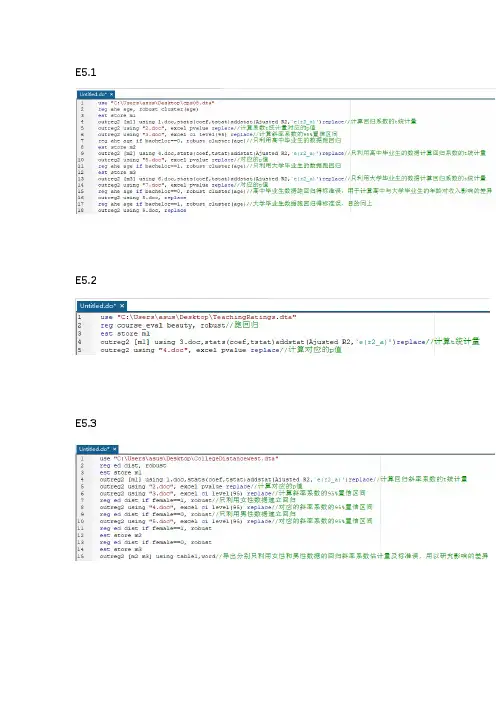
E5.2E5.3E6.2E6.3(1) VARIABLES ahe age 0.605*** (1.40e-09) Constant 1.082 (0.150) Observations 7,711 R-squared 0.029Robust pval in parentheses *** p<0.01, ** p<0.05, * p<0.1Robust t-statistics in parentheses *** p<0.01, ** p<0.05, * p<0.1a. 在对双边备择检验中，系数的t 统计量为24.70>2.58，与系数对应的p 值是0.0000000014趋近于0<0.01，所以可以在1%显著水平下拒绝原假设，自然可以在5%、10%水平下拒绝原假设。

(1) VARIABLES ahe age 0.605*** (0.550 - 0.660) Constant 1.082 (-0.473 - 2.638) Observations 7,711 R-squared 0.029Robust ci in parentheses *** p<0.01, ** p<0.05, * p<0.1b. 斜率系数95%的置信区间是(0.550，0.660)m1 VARIABLES ahe age 0.605*** (24.70) Constant 1.082 (1.574) Observations 7,711 R-squared 0.029 Ajusted R2 0.0289(1) m2 VARIABLES aheage 0.298***(7.513)Constant 6.522***(5.585)Observations 4,002R-squared 0.012Ajusted R2 0.0117Robust t-statistics in parentheses Robust pval in parentheses *** p<0.01, ** p<0.05, * p<0.1 *** p<0.01, ** p<0.05, * p<0.1只利用高中毕业生的数据，系数的t 统计量为7.513>2.58，与系数对应的p 值是0.0000364趋近于0<0.01，所以可以在1%显著水平下拒绝原假设，自然可以在5%、10%水平下拒绝原假设。

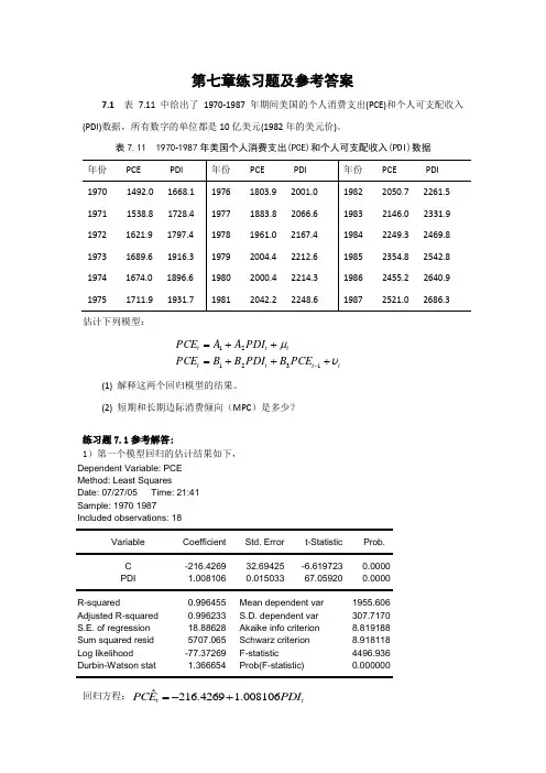
第七章练习题及参考答案7.1 表7.11中给出了1970-1987年期间美国的个人消费支出(PCE)和个人可支配收入(PDI)数据，所有数字的单位都是10亿美元(1982年的美元价)。

表7.11 1970-1987年美国个人消费支出(PCE)和个人可支配收入(PDI)数据估计下列模型：tt t t tt t PCE B PDI B B PCE PDI A A PCE υμ+++=++=-132121(1) 解释这两个回归模型的结果。

(2) 短期和长期边际消费倾向（MPC ）是多少？练习题7.1参考解答:1）第一个模型回归的估计结果如下，Dependent Variable: PCEMethod: Least Squares Date: 07/27/05 Time: 21:41 Sample: 1970 1987 Included observations: 18Variable Coefficient Std. Error t-StatisticProb. C -216.4269 32.69425 -6.619723 0.0000 PDI 1.008106 0.015033 67.05920 0.0000 R-squared 0.996455 Mean dependent var1955.606 Adjusted R-squared 0.996233 S.D. dependent var 307.7170 S.E. of regression 18.88628 Akaike info criterion 8.819188 Sum squared resid 5707.065 Schwarz criterion 8.918118 Log likelihood -77.37269 F-statistic 4496.936 Durbin-Watson stat 1.366654 Prob(F-statistic)0.000000回归方程：ˆ216.4269 1.008106t tPCE PDI =-+（32．69425） （0.015033） t =（-6.619723） （67.05920） 2R =0.996455 F=4496.936 第二个模型回归的估计结果如下，Dependent Variable: PCEMethod: Least Squares Date: 07/27/05 Time: 21:51 Sample (adjusted): 1971 1987 Included observations: 17 after adjustmentsVariable Coefficient Std. Error t-Statistic Prob.C -233.2736 45.55736 -5.120436 0.0002 PDI 0.982382 0.140928 6.970817 0.0000 PCE(-1) 0.037158 0.144026 0.2579970.8002R-squared 0.996542 Mean dependent var 1982.876 Adjusted R-squared 0.996048 S.D. dependent var 293.9125 S.E. of regression 18.47783 Akaike info criterion 8.829805 Sum squared resid 4780.022 Schwarz criterion 8.976843 Log likelihood -72.05335 F-statistic 2017.064 Durbin-Watson stat 1.570195 Prob(F-statistic)0.000000回归方程：1ˆ233.27360.98240.0372t t t PCE PDI PCE -=-+- （45.557） （0.1409） （0.1440）t = （-5.120） （6.9708） （0.258） 2R =0.9965 F=2017.0642）从模型一得到MPC=1.008；从模型二得到，短期MPC=0.9824，由于模型二为自回归模型，要先转换为分布滞后模型才能得到长期边际消费倾向，我们可以从库伊克变换倒推得到长期MPC=0.9824/（1+0.0372）=0.9472。

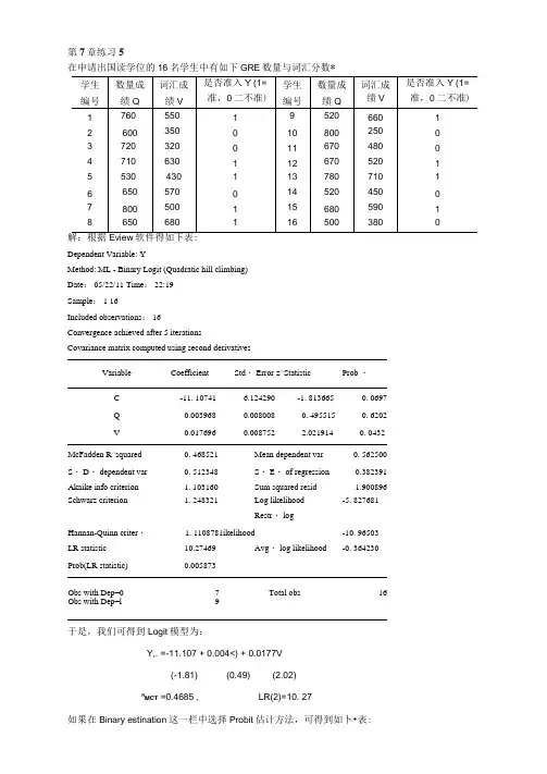
第7章练习5在申请出国读学位的16名学生中有如下GRE数量与词汇分数*EviewDependent Variable: YMethod: ML - Binary Logit (Quadratic hill climbing)Date： 05/22/11 Time： 22:19Sample： 1 16Included observations： 16Convergence achieved after 5 iterationsCovariance matrix computed using second derivativesVariable Coefficient Std・ Error z^Statistic Prob ・C -11. 10741 6.124290 -1. 813665 0. 0697Q 0.003968 0.008008 0. 495515 0. 6202V 0.017696 0.008752 2.021914 0. 0432 McFadden R^squared 0. 468521 Mean dependent var 0. 562500 S・ D・ dependent var 0. 512348 S・ E・ of regression 0.382391Akaike info criterion 1. 103160 Sum squared resid 1.900896 Schwarz criterion 1. 248321 Log likelihood -5. 827681Restr・ logHannan-Quinn criter・ 1. 1108781ikelihood -10. 96503 LR statistic 10.27469 Avg・ log likelihood -0. 364230 Prob(LR statistic) 0.005873Obs with Dep=0 7 Total obs 16 Obs with Dep=l 9于是，我们可得到Logit模型为：Y,. =-11.107 + 0.004<) + 0.0177V(-1.81) (0.49) (2.02)R MCT =0.4685 , LR(2)=10. 27如果在Binary estination这一栏中选择Probit估计方法，可得到如卜•表:Dependent Variable: YMethod: ML - Binary Probit (Quadratic hill climbing)Date： 05/22/11 Time： 22:25Sample： 1 16Included observations： 16Convergence achieved after 5 iterationsCovariance matrix computed using second derivativesVariable Coefficient Std・ Error z^Statistic Prob ・C -6. 634542 3.396882 -1. 953127 0. 0508Q 0.002403 0.001585 0. 524121 0. 6002V 0.010532 0.001693 2.244299 0. 0248McFadden R-squared 0.476272 Mean dependent var 0. 562500S・ D・ dependent var 0.512348 S・ E・ of regression 0.381655Akaike info criterion 1.092836 Sum squared resid 1.893588Schwarz criterion 1. 237696 Log likelihood -5.742687Restr・ logHannan-Quinn criter・ 1.100254 likelihood -10. 96503LR statistic 10. 44468 Avg・ log likelihood -0. 358918Prob(LR statistic) 0.005395Obs with Dep=0 7 Total obs 16Obs with Dep=l 9于是，我们可得到Probit模型为:Y； = -6.635 + 0.0024(2 + 0.0105V(-1.95) (0.52) (2.24)=0.4763 , LR(2)=10. 44第7章练习6下表列出了美国、加拿大、英国在1980^1999年的失业率Y以及对制造业的补偿X的相关数据资料。

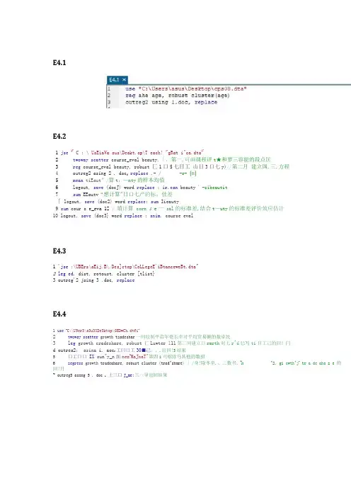
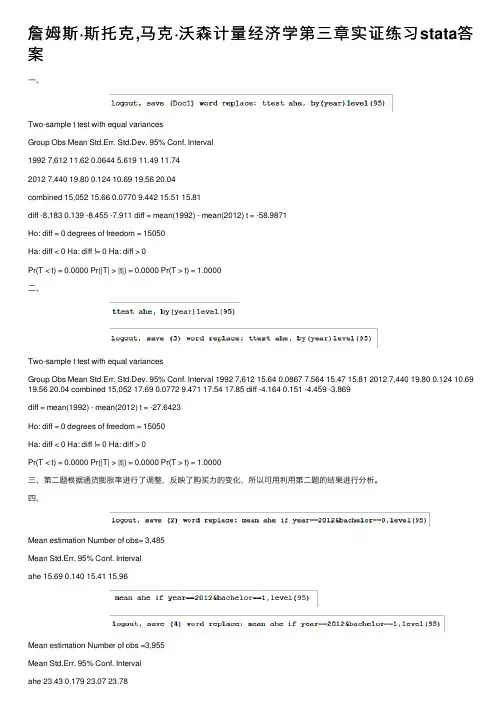
E4.1E4.21 jse 17 C : \ UsEiaVa sus\Deakt.op\T each! "gRat i"ca.dta172twoway scatter course_eval beauty.「，第一,可画课程评t★和萝三容能的段点匡3reg course_eval beauty, robust 匚1口5七日工山日3口七y)//第二月建立国.三.方程replace .- / -r- [H]4outreg2 asing 2 . docf5mean tiEaut”/算t：—nty的样本均值6logout, save (docJ) word replace : ir.ean beauty ;-zibeautit7sum EEautv“想计算"日口七产的标，佳差「logout, save (doc2) word replace: sum Iieauty9 sum cour s e_eva 1Z / 埴计算corn s e一sal的标准差,结合t―uty的标准差评价效应估计10 logout, save (doc3} word replace : snim. course evalE4.31 'jse :\UBErs\aEij.B\.Des]ctop\CoLLegeE'iBtanceweBt.dta"2leg ed. dist, rotoust. cluster [tlist}3 outreg'2 jsing 3 .doc, replaceE4.41 use n C:\U5er3\a3u3XDe3ktop\GEDwCh.dtfi w2twcway scatter growth tzadeshar一同绘制平启年亳长率对平均贸易额的敖卓民3leg growth cradeshare, robust 匚Luwter 111第三同建立口rmrth对七r^d巳写ti日工己的回！闩d outrea2；asina i. aoc工曰口工30■己，，.出回!3结果r5口工口口IX sun"y_n面ne=n MaJxaT"第四i司剔除马其他的数招6zegress growth tradeahare, robust cluater (trad^shmre) 」/身!除冬至.、二数书.~n^2. gi cwth^j-tr a de aha z e 的回!月~ outregS asxng 5 . doc t上三口J_me;三//导出回结果VARIABLES aheage 0.605(0.0245)Constant 1.082(0.688)Observations 7,711R-squared 0.029Robust standard errors in parentheses *** p<0.01, ** p<0.05, * p<0.11.① 截距估计值estimated intercept: 1,082② 斜率估计值estimated slope: 0,605回归方程：ahe= 1.082+0,605*age③当工人年长1岁，平均每小时工资增加0.605美元。

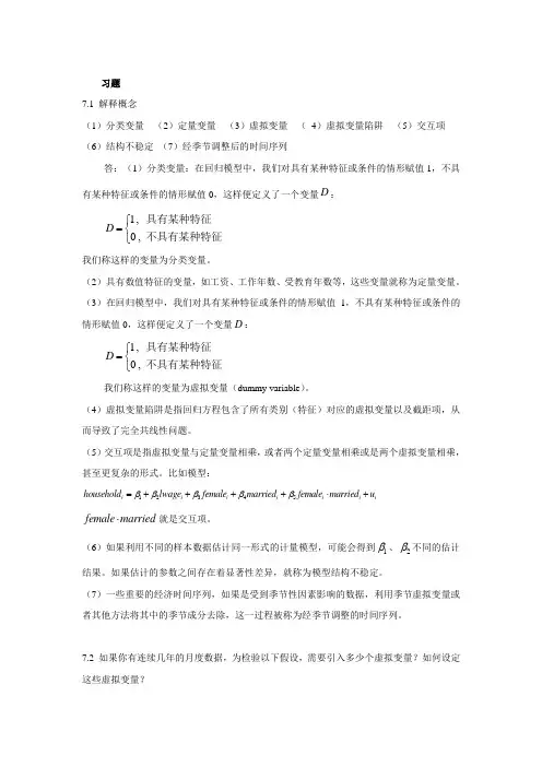
詹姆斯·斯托克,马克·沃森计量经济学第三章实证练习stata答案⼀、Two-sample t test with equal variancesGroup Obs Mean Std.Err. Std.Dev. 95% Conf. Interval1992 7,612 11.62 0.0644 5.619 11.49 11.742012 7,440 19.80 0.124 10.69 19.56 20.04combined 15,052 15.66 0.0770 9.442 15.51 15.81diff -8,183 0.139 -8.455 -7.911 diff = mean(1992) - mean(2012) t = -58.9871Ho: diff = 0 degrees of freedom = 15050Ha: diff < 0 Ha: diff != 0 Ha: diff > 0Pr(T < t) = 0.0000 Pr(|T| > |t|) = 0.0000 Pr(T > t) = 1.0000⼆、Two-sample t test with equal variancesGroup Obs Mean Std.Err. Std.Dev. 95% Conf. Interval 1992 7,612 15.64 0.0867 7.564 15.47 15.81 2012 7,440 19.80 0.124 10.69 19.56 20.04 combined 15,052 17.69 0.0772 9.471 17.54 17.85 diff -4.164 0.151 -4.459 -3.869diff = mean(1992) - mean(2012) t = -27.6423Ho: diff = 0 degrees of freedom = 15050Ha: diff < 0 Ha: diff != 0 Ha: diff > 0Pr(T < t) = 0.0000 Pr(|T| > |t|) = 0.0000 Pr(T > t) = 1.0000三、第⼆题根据通货膨胀率进⾏了调整，反映了购买⼒的变化，所以可⽤利⽤第⼆题的结果进⾏分析。

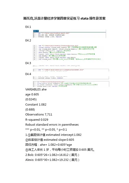
习题7.1 解释概念（1）分类变量 （2）定量变量 （3）虚拟变量 （ 4）虚拟变量陷阱 （5）交互项（6）结构不稳定 （7）经季节调整后的时间序列答：（1）分类变量：在回归模型中，我们对具有某种特征或条件的情形赋值1，不具有某种特征或条件的情形赋值0，这样便定义了一个变量D ：1,0,D ⎧=⎨⎩具有某种特征不具有某种特征我们称这样的变量为分类变量。

（2）具有数值特征的变量，如工资、工作年数、受教育年数等，这些变量就称为定量变量。

（3）在回归模型中，我们对具有某种特征或条件的情形赋值1，不具有某种特征或条件的情形赋值0，这样便定义了一个变量D ：1,0,D ⎧=⎨⎩具有某种特征不具有某种特征 我们称这样的变量为虚拟变量（dummy variable ）。

（4）虚拟变量陷阱是指回归方程包含了所有类别（特征）对应的虚拟变量以及截距项，从而导致了完全共线性问题。

（5）交互项是指虚拟变量与定量变量相乘，或者两个定量变量相乘或是两个虚拟变量相乘，甚至更复杂的形式。

比如模型：12345i i i i i i i household lwage female married female married u βββββ=++++⋅+female married ⋅就是交互项。

（6）如果利用不同的样本数据估计同一形式的计量模型，可能会得到1β、2β不同的估计结果。

如果估计的参数之间存在着显著性差异，就称为模型结构不稳定。

（7）一些重要的经济时间序列，如果是受到季节性因素影响的数据，利用季节虚拟变量或者其他方法将其中的季节成分去除，这一过程被称为经季节调整的时间序列。

7.2 如果你有连续几年的月度数据，为检验以下假设，需要引入多少个虚拟变量？如何设定这些虚拟变量？（1）一年中的每一个月份都表现出受季节因素影响；（2）只有2、7、8月表现出受季节因素影响。

答：（1）对于一年中的每个月份都受季节因素影响这一假设，需要引入三个虚拟变量。

斯托克,沃森计量经济学第四章实证练习stata操作及答案E4.1E4.2E4.3E4.4VARIABLES aheage 0.605(0.0245)Constant 1.082(0.688)Observations 7,711R-squared 0.029Robust standard errors in parentheses*** p<0.01, ** p<0.05, * p<0.11.①截距估计值estimated intercept:1.082②斜率估计值estimated slope:0.605回归方程：ahe= 1.082+0.605*age③当工人年长1岁，平均每小时工资增加0.605美元。

2.Bob: 0.605*26+1.082=16.812（美元）Alexis: 0.605*30+1.082=19.232（美元）答：预测Bob的收入为每小时16.812美元，Alexis为19.232美元。

3.年龄不能解释不同个体收入变化的大部分。

因为R-squared反映了因变量的全部变化能通过回归关系被自变量充分解释的比例，而分析得R-squared的值为0.029，解释度低，说明年龄不能解释不同个体收入变化的大部分。

1.答：两者看上去有微弱的正相关关系2.VARIABLES course_evalbeauty 0.133(0.0550)Constant 3.998(0.0449)Observations 463R-squared 0.036Robust standard errors in parentheses*** p<0.01, ** p<0.05, * p<0.1①截距估计值：3.998斜率估计值：0.133回归方程：Course_Eval=3.998+0.133*beauty//mean beautyMean estimation Number of obs = 463Mean Std.Err. 95% Conf. Interval beauty 4.75e-08 0.0367 -0.0720 0.0720②截距的估计值=Course_Eval的样本均值-斜率估计值*Beauty 的样本均值计算得Beauty的样本均值趋近于零，所以截距的估计值等于Course_Eval的样本均值。

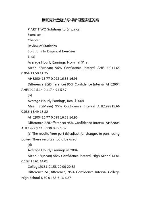
斯托克计量经济学课后习题实证答案P ART T WO Solutions to EmpiricalExercisesChapter 3Review of StatisticsSolutions to Empirical Exercises1. (a)Average Hourly Earnings, Nominal $’sMean SE(Mean) 95% Confidence Interval AHE199211.63 0.064 11.50 11.75AHE200416.77 0.098 16.58 16.96Difference SE(Difference) 95% Confidence Interval AHE2004 AHE1992 5.14 0.117 4.91 5.37(b)Average Hourly Earnings, Real $2004Mean SE(Mean) 95% Confidence Interval AHE199215.66 0.086 15.49 15.82AHE200416.77 0.098 16.58 16.96Difference SE(Difference) 95% Confidence Interval AHE2004 AHE1992 1.11 0.130 0.85 1.37(c) The results from part (b) adjust for changes in purchasing power. These results should be used.(d)Average Hourly Earnings in 2004Mean SE(Mean) 95% Confidence Interval High School13.81 0.102 13.61 14.01College20.31 0.158 20.00 20.62Difference SE(Difference) 95% Confidence Interval College High School 6.50 0.188 6.13 6.87Solutions to Empirical Exercises in Chapter 3 109(e)Average Hourly Earnings in 1992 (in $2004)Mean SE(Mean) 95% Confidence Interval High School13.48 0.091 13.30 13.65 College19.07 0.148 18.78 19.36Difference SE(Difference) 95% Confidence Interval College High School5.59 0.173 5.25 5.93(f) Average Hourly Earnings in 2004Mean SE(Mean) 95% Confidence Interval AHE HS ,2004AHE HS ,19920.33 0.137 0.06 0.60 AHE Col ,2004AHE Col ,19921.24 0.217 0.82 1.66Col–HS Gap (1992)5.59 0.173 5.25 5.93 Col–HS Gap (2004)6.50 0.188 6.13 6.87Difference SE(Difference) 95% Confidence Interval Gap 2004 Gap 1992 0.91 0.256 0.41 1.41Wages of high school graduates increased by an estimated 0.33 dollars per hour (with a 95%confidence interval of 0.06 0.60); Wages of college graduates increased by an estimated 1.24dollars per hour (with a 95% confidence interval of 0.82 1.66). The College High School gap increased by an estimated 0.91 dollars per hour.(g) Gender Gap in Earnings for High School Graduates Yearm Y s m n m w Y s w n w m Y w Y SE (m Y w Y )95% CI 199214.57 6.55 2770 11.86 5.21 1870 2.71 0.173 2.37 3.05 200414.88 7.16 2772 11.92 5.39 1574 2.96 0.192 2.59 3.34There is a large and statistically significant gender gap in earnings for high school graduates.In 2004 the estimated gap was $2.96 per hour; in 1992 the estimated gap was $2.71 per hour(in $2004). The increase in the gender gap is somewhat smaller for high school graduates thanit is for college graduates.Chapter 4Linear Regression with One RegressorSolutions to Empirical Exercises1. (a) ·AHE 3.32 0.45 u AgeEarnings increase, on average, by 0.45 dollars per hour when workers age by 1 year.(b) Bob’s predicted earnings 3.32 0.45 u 26 $11.70Alexis’s predicted earnings 3.32 0.45 u 30 $13.70(c) The R2 is 0.02.This mean that age explains a small fraction of the variability in earnings acrossindividuals.2. (a)There appears to be a weak positive relationship between course evaluation and the beauty index.Course Eval 4.00 0.133 u Beauty. The variable Beauty has a mean that is equal to 0; the(b) ·_estimated intercept is the mean of the dependent variable (Course_Eval) minus the estimatedslope (0.133) times the mean of the regressor (Beauty). Thus, the estimated intercept is equalto the mean of Course_Eval.(c) The standard deviation of Beauty is 0.789. ThusProfessor Watson’s predicted course evaluations 4.00 0.133 u 0 u 0.789 4.00Professor Stock’s predicted course evaluations 4.00 0.133 u 1 u 0.789 4.105Solutions to Empirical Exercises in Chapter 4 111(d) The standard deviation of course evaluations is 0.55 and the standard deviation of beauty is0.789. A one standard deviation increase in beauty is expected to increase course evaluation by0.133 u 0.789 0.105, or 1/5 of a standard deviation of course evaluations. The effect is small.(e) The regression R2 is 0.036, so that Beauty explains only3.6% of the variance in courseevaluations.3. (a) ?Ed 13.96 0.073 u Dist. The regression predicts that if colleges are built 10 miles closerto where students go to high school, average years of college will increase by 0.073 years.(b) Bob’s predicted years of completed education 13.960.073 u 2 13.81Bob’s predicted years of completed education if he was 10 miles from college 13.96 0.073 u1 13.89(c) The regression R2 is 0.0074, so that distance explains only a very small fraction of years ofcompleted education.(d) SER 1.8074 years.4. (a)Yes, there appears to be a weak positive relationship.(b) Malta is the “outlying” observation with a trade share of 2.(c) ·Growth 0.64 2.31 u TradesharePredicted growth 0.64 2.31 u 1 2.95(d) ·Growth 0.96 1.68 u TradesharePredicted growth 0.96 1.68 u 1 2.74(e) Malta is an island nation in the Mediterranean Sea, south of Sicily. Malta is a freight transportsite, which explains its larg e “trade share”. Many goods coming into Malta (imports into Malta)and immediately transported to other countries (as exports from Malta). Thus, Malta’s importsand exports and unlike the imports and exports of most other countries. Malta should not beincluded in the analysis.Chapter 5Regression with a Single Regressor:Hypothesis Tests and Confidence IntervalsSolutions to Empirical Exercises1. (a) ·AHE 3.32 0.45 u Age(0.97) (0.03)The t -statistic is 0.45/0.03 13.71, which has a p -value of 0.000, so the null hypothesis can berejected at the 1% level (and thus, also at the 10% and 5% levels).(b) 0.45 r 1.96 u 0.03 0.387 to 0.517(c) ·AHE 6.20 0.26 u Age(1.02) (0.03)The t -statistic is 0.26/0.03 7.43, which has a p -value of 0.000, so the null hypothesis can berejected at the 1% level (and thus, also at the 10% and 5% levels).(d) ·AHE 0.23 0.69 u Age(1.54) (0.05)The t -statistic is 0.69/0.05 13.06, which has a p -value of 0.000, so the null hypothesis can berejected at the 1% level (and thus, also at the 10% and 5% levels).(e) The difference in the estimated E 1 coefficients is 1,1,??College HighScool E E 0.69 0.26 0.43. Thestandard error of for the estimated difference is SE 1,1,??()College HighScoolE E (0.032 0.052)1/2 0.06, so that a 95% confidence interval for the difference is 0.43 r 1.96 u 0.06 0.32 to 0.54(dollars per hour).2. ·_ 4.000.13CourseEval Beauty u (0.03) (0.03)The t -statistic is 0.13/0.03 4.12, which has a p -value of 0.000, so the null hypothesis can be rejectedat the 1% level (and thus, also at the 10% and 5% levels).3. (a) ?Ed13.96 0.073 u Dist (0.04) (0.013)The t -statistic is 0.073/0.013 5.46, which has a p -value of 0.000, so the null hypothesis can be rejected at the 1% level (and thus, also at the 10% and 5% levels).(b) The 95% confidence interval is 0.073 r 1.96 u 0.013 or0.100 to 0.047.(c) ?Ed13.94 0.064 u Dist (0.05) (0.018)Solutions to Empirical Exercises in Chapter 5 113(d) ?Ed13.98 0.084 u Dist (0.06) (0.013)(e) The difference in the estimated E 1 coefficients is 1,1,??Female Male E E 0.064 ( 0.084) 0.020.The standard error of for the estimated difference is SE 1,1,??()Female Male E E (0.0182 0.0132)1/20.022, so that a 95% confidence interval for the difference is 0.020 r 1.96 u 0.022 or 0.022 to0.064. The difference is not statistically different.Chapter 6Linear Regression with Multiple RegressorsSolutions to Empirical Exercises1. Regressions used in (a) and (b)Regressor a bBeauty 0.133 0.166Intro 0.011OneCredit 0.634Female 0.173Minority 0.167NNEnglish 0.244Intercept 4.00 4.07SER 0.545 0.513R2 0.036 0.155(a) The estimated slope is 0.133(b) The estimated slope is 0.166. The coefficient does not change by an large amount. Thus, theredoes not appear to be large omitted variable bias.(c) Professor Smith’s predicted course evaluation (0.166 u 0)0.011 u 0) (0.634 u 0) (0.173 u0) (0.167 u 1) (0.244 u 0) 4.068 3.9012. Estimated regressions used in questionModelRegressor a bdist 0.073 0.032bytest 0.093female 0.145black 0.367hispanic 0.398incomehi 0.395ownhome 0.152dadcoll 0.696cue80 0.023stwmfg80 0.051intercept 13.956 8.827SER 1.81 1.84R2 0.007 0.279R0.007 0.277Solutions to Empirical Exercises in Chapter 6 115(a) 0.073(b) 0.032(c) The coefficient has fallen by more than 50%. Thus, it seems that result in (a) did suffer fromomitted variable bias.(d) The regression in (b) fits the data much better as indicated by the R2, 2,R and SER. The R2 and R are similar because the number of observations is large (n 3796).(e) Students with a “dadcoll 1” (so that the student’s father went to college) complete 0.696 moreyears of education, on average, than students with “dadcoll 0” (so that the student’s father didnot go to college).(f) These terms capture the opportunity cost of attending college. As STWMFG increases, forgonewages increase, so that, on average, college attendance declines. The negative sign on thecoefficient is consistent with this. As CUE80 increases, it is more difficult to find a job, whichlowers the opportunity cost of attending college, so that college attendance increases. Thepositive sign on the coefficient is consistent with this.(g) Bob’s predicted years of education 0.0315 u 2 0.093 u58 0.145 u 0 0.367 u 1 0.398 u0 0.395 u 1 0.152 u 1 0.696 u 0 0.023 u 7.5 0.051 u 9.75 8.82714.75(h) Jim’s expected years of education is 2 u 0.0315 0.0630 less than Bob’s. Thus, Jim’s expectedyears of education is 14.75 0.063 14.69.3.Variable Mean StandardDeviation Unitsgrowth 1.86 1.82 Percentage Pointsrgdp60 3131 2523 $1960tradeshare 0.542 0.229 unit freeyearsschool 3.95 2.55 yearsrev_coups 0.170 0.225 coups per yearassasinations 0.281 0.494 assasinations per yearoil 0 0 0–1 indicator variable (b) Estimated Regression (in table format):Regressor Coefficienttradeshare 1.34(0.88)yearsschool 0.56**(0.13)rev_coups 2.15*(0.87)assasinations 0.32(0.38)rgdp60 0.00046**(0.00012)intercept 0.626(0.869)SER 1.59R2 0.29R0.23116 Stock/Watson - Introduction to Econometrics - Second EditionThe coefficient on Rev_Coups is í2.15. An additional coup in a five year period, reduces theaverage year growth rate by (2.15/5) = 0.43% over this 25 year period. This means the GPD in 1995 is expected to be approximately .43×25 = 10.75% lower. This is a larg e effect.(c) The 95% confidence interval is 1.34 r 1.96 u 0.88 or 0.42 to 3.10. The coefficient is notstatistically significant at the 5% level.(d) The F-statistic is 8.18 which is larger than 1% critical value of 3.32.Chapter 7Hypothesis Tests and Confidence Intervals in Multiple RegressionSolutions to Empirical Exercises1. Estimated RegressionsModelRegressor a bAge 0.45(0.03)0.44 (0.03)Female 3.17(0.18)Bachelor 6.87(0.19)Intercept 3.32(0.97)SER 8.66 7.88R20.023 0.1902R0.022 0.190(a) The estimated slope is 0.45(b) The estimated marginal effect of Age on AHE is 0.44 dollars per year. The 95% confidenceinterval is 0.44 r 1.96 u 0.03 or 0.38 to 0.50.(c) The results are quite similar. Evidently the regression in (a) does not suffer from importantomitted variable bias.(d) Bob’s predicted average hourly earnings 0.44 u 26 3.17 u 0 6.87 u 0 3.32 $11.44Alexis’s predicted average hourly earnings 0.44 u 30 3.17 u 1 6.87 u 1 3.32 $20.22 (e) The regression in (b) fits the data much better. Gender and education are important predictors of earnings. The R2 and R are similar because the sample size is large (n 7986).(f) Gender and education are important. The F-statistic is 752, which is (much) larger than the 1%critical value of 4.61.(g) The omitted variables must have non-zero coefficients and must correlated with the includedregressor. From (f) Female and Bachelor have non-zero coefficients; yet there does not seem to be important omittedvariable bias, suggesting that the correlation of Age and Female and Age and Bachelor is small. (The sample correlations are ·Cor(Age, Female) 0.03 and·Cor(Age,Bachelor) 0.00).118 Stock/Watson - Introduction to Econometrics - Second Edition2.ModelRegressor a b cBeauty 0.13**(0.03) 0.17**(0.03)0.17(0.03)Intro 0.01(0.06)OneCredit 0.63**(0.11) 0.64** (0.10)Female 0.17**(0.05) 0.17** (0.05)Minority 0.17**(0.07) 0.16** (0.07)NNEnglish 0.24**(0.09) 0.25** (0.09)Intercept 4.00**(0.03) 4.07**(0.04)4.07**(0.04)SER 0.545 0.513 0.513R2 0.036 0.155 0.1552R0.034 0.144 0.145(a) 0.13 r 0.03 u 1.96 or 0.07 to 0.20(b) See the table above. Intro is not significant in (b), but the other variables are significant.A reasonable 95% confidence interval is 0.17 r 1.96 u 0.03 or0.11 to 0.23.Solutions to Empirical Exercises in Chapter 7 119 3.ModelRegressor (a) (b) (c)dist 0.073**(0.013) 0.031**(0.012)0.033**(0.013)bytest 0.092**(0.003) 0.093** (.003)female 0.143**(0.050) 0.144** (0.050)black 0.354**(0.067) 0.338** (0.069)hispanic 0.402**(0.074) 0.349** (0.077)incomehi 0.367**(0.062) 0.374** (0.062)ownhome 0.146*(0.065) 0.143* (0.065)dadcoll 0.570**(0.076) 0.574** (0.076)momcoll 0.379**(0.084) 0.379** (0.084)cue80 0.024**(0.009) 0.028** (0.010)stwmfg80 0.050*(0.020) 0.043* (0.020)urban 0.0652(0.063) tuition 0.184(0.099)intercept 13.956**(0.038) 8.861**(0.241)8.893**(0.243)F-statitisticfor urban and tuitionSER 1.81 1.54 1.54R2 0.007 0.282 0.284R0.007 0.281 0.281(a) The group’s claim is that the coefficien t on Dist is 0.075 ( 0.15/2). The 95% confidence forE Dist from column (a) is 0.073 r 1.96 u 0.013 or 0.099 to 0.046. The group’s claim is includedin the 95% confidence interval so that it is consistent with the estimated regression.120 Stock/Watson - Introduction to Econometrics - Second Edition(b) Column (b) shows the base specification controlling for other important factors. Here thecoefficient on Dist is 0.031, much different than the resultsfrom the simple regression in (a);when additional variables are added (column (c)), the coefficient on Dist changes little from the result in (b). From the base specification (b), the 95% confidence interval for E Dist is0.031 r1.96 u 0.012 or 0.055 to 0.008. Similar results are obtained from the regression in (c).(c) Yes, the estimated coefficients E Black and E Hispanic are positive, large, and statistically significant.Chapter 8Nonlinear Regression FunctionsSolutions to Empirical Exercises1. This table contains the results from seven regressions that are referenced in these answers.Data from 2004(1) (2) (3) (4) (5) (6) (7) (8)Dependent VariableAHE ln(AHE) ln(AHE) ln(AHE) ln(AHE) ln(AHE) ln(AHE) ln(AHE) Age 0.439**(0.030) 0.024**(0.002)0.147**(0.042)0.146**(0.042)0.190**(0.056)0.117*(0.056)0.160Age2 0.0021**(0.0007) 0.0021** (0.0007)0.0027**(0.0009)0.0017(0.0009)0.0023(0.0011)ln(Age) 0.725**(0.052)Female u Age 0.097 (0.084) 0.123 (0.084) Female u Age2 0.0015 (0.0014)0.0019 (0.0014) Bachelor u Age 0.064 (0.083)0.091 (0.084) Bachelor u Age2 0.0009 (0.0014) 0.0013 (0.0014) Female 3.158**(0.176) 0.180**(0.010)0.180**(0.010)0.180**(0.010)(0.014)1.358*(1.230)0.210**(0.014)1.764(1.239)Bachelor 6.865**(0.185) 0.405**(0.010)0.405**(0.010)0.405**(0.010)0.378**(0.014)0.378**(0.014)0.769(1.228)1.186(1.239)Female u Bachelor 0.064** (0.021) 0.063**(0.021)0.066**(0.021)0.066**(0.021)Intercept 1.884(0.897) 1.856**(0.053)0.128(0.177)0.059(0.613)0.078(0.612)0.633(0.819)0.604(0.819)0.095(0.945)F-statistic and p-values on joint hypotheses(a) F-statistic on terms involving Age 98.54(0.00)100.30(0.00)51.42(0.00)53.04(0.00)36.72(0.00)(b) Interaction termswithAge24.12(0.02)7.15(0.00)6.43(0.00)SER 7.884 0.457 0.457 0.457 0.457 0.456 0.456 0.456 R0.1897 0.1921 0.1924 0.1929 0.1937 0.1943 0.1950 0.1959 Significant at the *5% and **1% significance level.122 Stock/Watson - Introduction to Econometrics - Second Edition(a) The regression results for this question are shown in column (1) of the table. If Age increasesfrom 25 to 26, earnings are predicted to increase by $0.439 per hour. If Age increases from33 to 34, earnings are predicted to increase by $0.439 per hour. These values are the samebecause the regression is a linear function relating AHE and Age .(b) The regression results for this question are shown in column (2) of the table. If Age increasesfrom 25 to 26, ln(AHE ) is predicted to increase by 0.024. This means that earnings are predicted to increase by 2.4%. If Age increases from 34 to 35, ln(AHE ) is predicted to increase by 0.024.This means that earnings are predicted to increase by 2.4%. These values, in percentage terms,are the same because the regression is a linear function relating ln(AHE ) and Age .(c) The regression results for this question are shown in column (3) of the table. If Age increasesfrom 25 to 26, then ln(Age ) has increased by ln(26) ln(25) 0.0392 (or 3.92%). The predictedincrease in ln(AHE ) is 0.725 u (.0392) 0.0284. This means that earnings are predicted toincrease by 2.8%. If Age increases from 34 to 35, then ln(Age ) has increased by ln(35) ln(34) .0290 (or 2.90%). The predicted increase in ln(AHE ) is 0.725 u (0.0290) 0.0210. This means that earnings are predicted to increase by 2.10%.(d) When Age increases from 25 to 26, the predicted change in ln(AHE ) is(0.147 u 26 0.0021 u 262) (0.147 u 25 0.0021 u 252) 0.0399.This means that earnings are predicted to increase by 3.99%.When Age increases from 34 to 35, the predicted change in ln(AHE ) is(0. 147 u 35 0.0021 u 352) (0. 147 u 34 0.0021 u 342) 0.0063.This means that earnings are predicted to increase by 0.63%.(e) The regressions differ in their choice of one of the regressors. They can be compared on the basis of the .R The regression in (3) has a (marginally) higher 2,R so it is preferred.(f) The regression in (4) adds the variable Age 2 to regression(2). The coefficient on Age 2 isstatistically significant ( t 2.91), and this suggests that the addition of Age 2 is important. Thus,(4) is preferred to (2).(g) The regressions differ in their choice of one of the regressors. They can be compared on the basis of the .R The regression in (4) has a (marginally) higher 2,R so it is preferred.(h)Solutions to Empirical Exercises in Chapter 8 123 The regression functions using Age (2) and ln(Age) (3) are similar. The quadratic regression (4) is different. It shows a decreasing effect of Age on ln(AHE) as workers age.The regression functions for a female with a high school diploma will look just like these, but they will be shifted by the amount of the coefficient on the binary regressor Female. The regression functions for workers with a bachelor’s degree will also look just like these, but they would be shifted by the amount of the coefficient on the binary variable Bachelor.(i) This regression is shown in column (5). The coefficient on the interaction term Female uBachelor shows the “extra effect” of Bachelor on ln(AHE) for women relative the effect for men.Predicted values of ln(AHE):Alexis: 0.146 u 30 0.0021 u 302 0.180 u 1 0.405 u 1 0.064 u 1 0.078 4.504Jane: 0.146 u 30 0.0021 u 302 0.180 u 1 0.405 u 0 0.064 u 0 0.078 4.063Bob: 0.146 u 30 0.0021 u 302 0.180 u 0 0.405 u 1 0.064 u 0 0.078 4.651Jim: 0.146 u 30 0.0021 u 302 0.180 u 0 0.405 u 0 0.064 u 0 0.078 4.273Difference in ln(AHE): Alexis Jane 4.504 4.063 0.441Difference in ln(AHE): Bob Jim 4.651 4.273 0.378Notice that the difference in the difference predicted effects is 0.441 0.378 0.063, which is the value of the coefficient on the interaction term.(j) This regression is shown in (6), which includes two additional regressors: the interactions of Female and the age variables, Age and Age2. The F-statistic testing the restriction that the coefficients on these interaction terms is equal to zero is F 4.12 with a p-value of 0.02. This implies that there is statistically significant evidence (at the 5% level) that there is a different effect of Age on ln(AHE) for men and women.(k) This regression is shown in (7), which includes two additional regressors that are interactions of Bachelor and the age variables, Age and Age2. The F-statistic testing the restriction that the coefficients on these interaction terms is zero is 7.15 with a p-value of 0.00. This implies that there is statistically significant evidence (at the 1% level) that there is a different effect of Age on ln(AHE) for high school and college graduates.(l) Regression (8) includes Age and Age2 and interactions terms involving Female and Bachelor.The figure below shows the regressions predicted value of ln(AHE) for male and females with high school and college degrees.124 Stock/Watson - Introduction to Econometrics - Second EditionThe estimated regressions suggest that earnings increase as workers age from 25–35, the rangeof age studied in this sample. There is evidence that the quadratic term Age2 belongs in theregression. Curvature in the regression functions in particularly important for men.Gender and education are significant predictors of earnings, and there are statistically significant interaction effects between age and gender and age and education. The table below summarizes the regressions predictions for increases in earnings as a person ages from 25 to 32 and 32 to 35Gender, Education Predicted ln(AHE) at Age(Percent per year)25 32 35 25 to 32 32 to 35Males, High School 2.46 2.65 2.67 2.8% 0.5%Females, BA 2.68 2.89 2.93 3.0% 1.3%Males, BA 2.74 3.06 3.09 4.6% 1.0%Earnings for those with a college education are higher than those with a high school degree, andearnings of the college educated increase more rapidly early in their careers (age 25–32). Earnings for men are higher than those of women, and earnings of men increase more rapidly early in theircareers (age 25–32). For all categories of workers (men/women, high school/college) earningsincrease more rapidly from age 25–32 than from 32–35.。