优选Ch随机变量序列的极限

Chapter 8 Random Variable8.1 What is a random variable?A random variable (abbreviation: r.v.) assigns a number value to each outcome (simple event, sample point) of a random circumstance. e.g. Toss a die and observe the number of face upRandom variables is denoted by X, Y (or X(ω), when a specific simple eventωis emphasized)●A continuous random variable can takeany value in an interval or a collectionof intervals●A discrete random variable can takeone of a countable list of distinct values 8.2 Discrete random variableExamples1. (Toss a fair coin –the random circumstance)X = the number of times the “head” occurs Then X can take 1(“head”occurs) or 0 (“tail” occurs)2. X = # of defectives in a package of 50 cellphones3. Y = # of calls needed to get through in a fixed time period4. Repeatedly tossing a fair coin, and define the r.v.:X =number of tosses until the head occursThe Probability Distribution of discrete random variablesThe Probability Distribution Function (pdf ) of a discrete r.v. X is a table ，or a rule that assigns probability )(i i x X P p ==to the possible values i x of the r.v. X , denoted by),(~1p 1p 0p p x x X i ii i 1i 1=<<⎪⎪⎭⎫ ⎝⎛∑ The pdf describes completely the probabilistic rule of a discrete r.v.In Example 4, one has P(X =k ) = k21⎪⎭⎫ ⎝⎛, i.e. ⎪⎪⎭⎫ ⎝⎛ k 2121k 1X ~Miniproblem What about tossing a biased coin, where the probability of occurring head is p8.3 Expected value (Mean) for a discrete r.v. Expected value (Expectation ) of a discrete r.v. X , denoted by EX , is a weighted average value of X :i i ip x EX ∑=, which is exactly the Mean value of X , Usually μ is used to represent EX● Describing the central tendency of pdf ● Weighted average of all possible values ● Approximated by the average when the experiment is repeated independently a very large number of timesStandard Deviation for a discrete r.v. Variance of X :i 2i i 2denoteby 2definedby p x EX X E X V )()()(μσ-==-=∑● Weighted average squared deviation fromthe meanStandard Deviation of X : σ=)(X VMeasures the variability of the distributionExample 8.7The randomized schedule I and II are employed respectively for investing $100 Net gains after 1 year for I and for II are⎪⎪⎭⎫ ⎝⎛994005001010005000X 1...$$$~,⎪⎪⎭⎫ ⎝⎛52341020X 2...$$$~. Then10EX EX 21$==,936X V 92172X V 21.$)(,.$)(==Plan II sounds better.8. 4 Binomial Random VariablesBinomial Experiments and Binomial r.v. Binomial Experiment characteristics: ● Sequence of n identical trials● Each trial has 2 outcomes: S(‘Success’) or F(‘failure’)● The probability of success of each trial is p● Trials are independentBinomial r.v.:X = number of S in the n trials Examples⏹# of games Gophers won in the last season ⏹# of defective items in a batch of 5 items ⏹# of correct on a 33 questions quiz ⏹# of customers who purchase out of 100 customers who enter storeThe Probability for Binomial r.v.For a Binomial r.v. X , one hasP (X=k )),()!(!!p 1q n k 0q p k n k n k n k -=≤≤-=-That showsX ~⎪⎪⎭⎫ ⎝⎛--n k n k n p q p k n k n q n k 0 )!(!!, where we say that X has a binomial distribution , and denote it by X ~B(n , p )Microsoft Excel Tips : Calculating P(X=k ) by BINOMDIST(k,n,p,false ) P(X ≤k ) by BINOMDIST(k,n,p,true )(“false ” stands for exactly k successes, “true ” indicates for a cumulative probability)Tendency (Mean) & Standard Deviation of B (n,p ))()(,p 1np X V np EX -==More ExamplesRandom circumstance r.v. distributionToss 3 fair coins, #of H B (3,21)Roll a die 8 times #of 4 or 6 B (8,31)Randomly sample #of seeing B (1000,p ) 1000 US adults UFO p =proportionRoll 2 dies once Sum is 7 B (1, 366)MiniproblemYou t oss 2 coins. You’re interested in the number of tails. What are the expected value & standard deviation of this random variable, number of tails?8.5 Continuous random variables● Infinite number of outcomes in interval, too many to list like discrete variable● Probabilities of taking any special values are 0.ExamplesX = length of time between customer arrivalsSo are height, time, weight, monetary valuesProbability Density FunctionDiffer from determining the probability, we are only able to find the probability that X falls between two values and do this by determining the area between the two values under a curve f(x), called the Probability Density Function of the r.v. X.i.e. f(x) is a probability density function of X, if for any c, d, we have)()(dXcPdXcP<<=≤≤=Area under the curve f(x) between c and df(x) is not probability , but density(密度)hh xXxPxfh )(lim)(+≤≤=→Continuous Random Variable Accumulated Probability Function F(x)=)(XF Area under the curve f(x) between -∞and xExpected value (Mean) and Variance Mean of X :EX =μ = 纵坐标在概率密度函数f (x )与0间,横坐标在),(∞-∞的面积片在横坐标x 处加一个大小为x 的力(如x 值为负, 则表示反向的力), 所得的平衡点的横坐标Variance of X :22EX X E X V σ=-=)()(Standard Deviation of X : σ=)(X V ( 附注 FormulaMean ⎰=dx x xf )(μVariance ⎰-=dx x f x 22)()(μσ )x f x fBasic Rules)()(,)(X V c X V c EX c X E =++=+ )()(,)(X V c cX V cEX cX E 2== StandardizedIf μ=EX , 2X V σ=)( , then0X E =⎪⎭⎫ ⎝⎛-σμ,1X V =⎪⎭⎫ ⎝⎛-σμ where σμ-X is called the Standardized Error of X (随机变量X 对于其均值的无量纲化的随机偏差)Uniform Distribution(均匀分布)If a r.v. X takes equally likely outcomes in interval [c , d ], which is equivalent to that the probability density function f (x ) of X has the form of⎪⎩⎪⎨⎧≤≤-=)()()(otherwise 0d x c if c d 1x f ,then X is said to submit a uniformdistribution on the interval [c , d ], and denoted by X ~U [c , d ]Example 8.13 If you arrive at a bus stop randomly, where the bus comes every 10 minutes. Let X =waiting time until the next bus arrives. Then X ~U [0,10]. The probability that the waiting time between 5 and 7 minutes isP (5 ≤≤X 7) = Base ⨯Height= (7 - 5) 101⨯ = 51Another exampleYou’re the production manager of a soft drink bottling company. You believe that when a machine is set to dispense 12 oz., it really dispenses 11.5 to 12.5 oz. inclusive. Suppose the amount dispensed has a uniform distribution. What is the probability that less than 11.8 oz. is dispensed?Solution: A randomly drawn machine is set to dispense X oz. Then X ~ U [11.5,12.5], andP (11.5 ≤≤X 11.8) = Base ⨯Height = (11.8 - 11.5) ⨯ 1 = 0.30Mean & standard deviation of Uniform r.v.s2d c +=μ,12c d 22)(-=σNormal DistributionProbability Density FunctionWe say that r.v. X submit Normal distribution with parameters2σμ,, if its probability density function has the form off(x) =2x21e21⎪⎭⎫⎝⎛--σμσπ, (0>σ),denoted by X ~N(2σμ,) .The calculation shows that the total area under the above curve is 1.Characters●Mean, median, mode are equal ( =μ)●σis the standard deviation of therandom variable X, which has infinite range, but effective width is 6 σThe area of the following shadow is 0.95 and the area between μ-3σ and μ+3σ is 0.997Effect of Varying Parameters (μ, 2σ)Small 2σ large 2σUsing probability Tables (Reducing to the Standard Normal Distribution N (0,1)) to calculate● If X is a normal r.v. , then aX +b is also anormal r.v. i.e. if),(~2N X σμ, then 22~(,)aX b N a b a μσ++ ● If X ~N (2σμ,), then σμ-X ~N (0,1)(Explain : change mean μ and standard deviation σ into 0 and 1. The value of σμ-=X Z is called z-score in statistics)Numerical Table of function Φ(z ) -- Cumulative Probability Function of the standard Normal Distribution (dx e 21z 2x 21z-∞-⎰=πΦ)() (标准正态分布累积概率函数的数值表: p.538-)(We have 500z 1z .)(),()(=-=-ΦΦΦ)A part of the value of Φ(z)-1/2 is shown asz ):Using z-score to solve problemsExampleP(3.8 ≤ X ≤ 5)= P(0.12 ≤ Z ≤ 0)).()(1200--=ΦΦ0478050120120150..).()].([.=-=--=ΦΦ Example),(~1005N X , then σμ-=X Z and).().().().(210301058Z 10517P 8X 17P ΦΦ-=-≤≤-=≤≤Real exampleYou work in Quality Control for GE. Light bulb life has a normal distribution with mean 2000 hours and standarddeviation 200 hours. What’s the probability that a bulb will last1. between 2000 & 2400 hours?2. less than 1470 hours?477222400X2000P.)()()(=-=≤≤ΦΦ00465216521470XP.).().()(=-=-=≤ΦΦMini-problem 1 (Reliability)Life testing has revealed that a particular type of TV picture tube has a length of life that is approximately normally distributed with a mean of 8000 hours and a standard deviation of 1000 hours. The manufacturer wants to set a guarantee period for the tube that will obligate the manufacturer to replace no more than 5% of all tubes sold. How long should the guarantee period be? Finding Percentiles (百分点)The 25th percentile x of a Normal r.v. isthe value having z-score zσμ-=xsatisfying 250z .)(=Φ. e.g. if the 25th percentile of pulse rate is 64, then there are 25% people has pulse rate below 64.The same way, the p -th percentile x is determined by 100p x =-)(σμΦ Microsoft Excel TipsNORMSDIST(z ) provides )(z ΦNORMSINV(p ) provides z satisfying p z =)(Φ8.7 Approximating Binomial Distribution ProbabilitiesNormal Approximation of a Binomial r.v.:A B (n , p ) r.v. X is approximately to follow the distribution N (np , np (1-p )), i.e. the N (EX , V(X))(Or say, )1(p np npX -- - the standardize of X , isapproximated by the standard normal distribution as n goes to infinite)Example 8.18 Number of Heads in 30 Flips of a fair coin ( B (30, 0.5))The Histogram looks quite like the density function of N (15,7.5)Approximating Cumulative Probabilitiesfor Binomial r.v.s()X np k np k np P X k P ---≤=≤≈ΦPractically, this approximation is applied when both np and n(1-p) are at least 5, and usually at least 10 is preferable8.8 Sums, difference, and Combinations of r.v.A linear combination of r.v. X ,Y ,…means aX+bY+…(including X+Y and X-Y ). ● Rule 1 E (aX+bY+…)=aEX+bEY+… ● Rule 2 If X ,Y ,…are independent , thenV (aX+bY+…)=2a V (X )+ 2b V (Y )+…● Warning: V (-X )(≠-V (X ))=V(X ) Combining Independent Normal r.v.sIf X ,Y are independent, and ),(~2X X N X σμ,),(~2Y Y N Y σμ, then ),(~2Y 2X Y X N Y X σσμμ+++Example (Missing flight or not)Meg leaves home 45 minutes before the last call for her flight will occur. Assume the driving time (minutes) ),(~925N X and the airport time ),(~415N Y , then the probability of missing her flight is))(()(49251545Z P 45Y X P ++->=>+082303911391Z P .).().(=-=>=ΦAdding Binomial r.v.s with the same Success probabilityIf X ,Y are independent, and ),(~p n B X X , ),(~p n B Y Y , then ),(~p n n B Y X Y X ++Example 8.23Strategies for Exam when out of timeTwo-part multiple-choice test with 10 questions in each part and having 4 choices for each question. You need get 13 questions or more right to pass. However, you don ’t have time to study all the materials. Fromexperience you know that if you study all the 20 questions well, then you can narrow all questions into 2 choices. If you study the first part carefully, then you will get right for these questions with probability 0.8, but you have to guess completely the other part. How can you do?Solution: you haveStrategy 1 - Study all the material wellLet S be the scores you will get, then,(=)),S=~,(.,10VS5ES520Ns.d. (standard deviation) =5= 2.24P≤S-=≥=131)((12SP)1- BINOMDIST(12,20,0.5,true) =0.1316 Strategy 2 - Study first part material only Let X and Y be the scores you will get for the part 1 and part 2 respectively, then X and Y are independent and,X.()(=,~=.,),EXX1NV68108(Y.),)(N=~=.,,.VY1105875225EY)(,.+)+=(=VY3475X25XY10E.s.d. of X +Y =473.= 1.86)(13Y X P ≥+is tedious to calculate, since Y X + no more follows the binomial distribution, but )(13Y X P ≥+can be estimated by simulation, which is, e.g. done 1000 times by randomly generating values of X +Y . e.g. there are 130 times of them not smaller than 13. Then we have 13013Y X P .)(≈≥+Conclusion: Neither one looks betterExponential Distribution⎩⎨⎧<≥=-)()()(0x 00x e x f xλλ,denoted by X ~exp λMean: EX =λ1, Variance: V (X ) = 21λConclusion of this chapter● Defined discrete and continuous random variable● Described the binomial, uniform, normal,& exponential random variables●Calculated probabilities for continuous random variable●Exploiting the normal approximation of the binomial distributionExercise of 7th week1. Mini-problem 12. A volunteer organization wants to find donors. 3volunteers agree to call potential donors. In past, about 20%of those called agreed independently to make a donation. If the 3volunteers make 10, 12and 18calls respectively, what is the probability that they get at least 10 donors?3. Alice and Julie each swam a mile a day. Alice’s times are normally distributed with mean =37 minutes and standard deviation =1 minute. Julie is faster but less consistent than Alice, and her times are normally distributed with mean =33minutes andstandard deviation =2 minutes. Their times are independent each other. Can Alice ever win?4. The standard medical treatment for a certain disease is successful in 60% of all cases.(1)The treatment is given to n =200 patients. What is the probability that the treatment is successful for 70% or more of these 200 patients?(2)How about the case of n=205 设),(~p n B X （二项分布）．分别对于 12108n ,,=及902010p .,,.,. =，n 10k ,,, =，作出k n k k np 1p C k X P --==)()(的数值表． (若用Matlab ，则要求给出程序与数值表；如用Execel 则要求写出计算的要领与注释（傻瓜化！））6. The number of training units that must be passed before a complex computer software program is mastered varies from one to five, depending on the student. After much experience, the software manufacturer has determined the probability distribution that describes the fraction of usersmastering the software after each number of training units:a. Calculate mean μ, variance σ2, and the standard deviation σ. Interpret μ in the context of the problem.b. Graph p(x). What is the probability that X is in the interval (μ–2σ, μ+2σ )?c. If the firm wants to ensure that at least 70% of the students master the program, what is the minimum number of training units that must be administered?7. A weather forecaster predicts that May rainfall in a local area will be between 3 and 6 cm but has no idea where the amount will be within that interval. Let X be the amount of May rainfall in the local area, and assume that X is uniformly distributed in the interval of 3 to 6 cma. State the density function of X and plot it on a graph.b. Obtain the mean and the standard deviation of the probability distribution.c. What is the probability that the observed Mayrainfall will be less than 5 cm?8. Gauges are used to reject all packages crackerwhere a certain weight is not within the specificationoz. It is know that this weight is normally 225ddistributed with mean 225oz. and variance 441 squareoz. Determine the value d such that the specificationscover 95% of the weight.9. The average life of a certain type of small motor is10 years with standard deviation of 2 years. Assumethat the lifetime of a motor follows a normaldistribution. The manufacturer replaces free allmotors that fail while under guarantee. If he is willingto replace only 3% of the motors that fail, how long aguarantee should he offer?10. The IQs of 600 applicants of a certain college areapproximately normally distributed with a mean of115and a standard deviation of 12. If the collegerequires an IQ at least 95, how many of these studentswill be rejected on this basis regardless of theirqualification?11. The safety jackets produced by a manufacturerhave rating with an average 840newtons(unit of the force) and a standard deviation 15newtons. Suppose that it follows normal distribution. To check whether the process is operating correctly, a manager takes a sample of 100jackets, rates them, and calculates the bar graph, the mean rating for jackets in the sample.(1) What is the probability that the sample mean is less than or equal to 830 newtons?(2) Suppose that on one particular day, the manager observed sample mean = 830. Would you conclude that this indicates that the true process mean for that day is still 840 newtons? Why?。

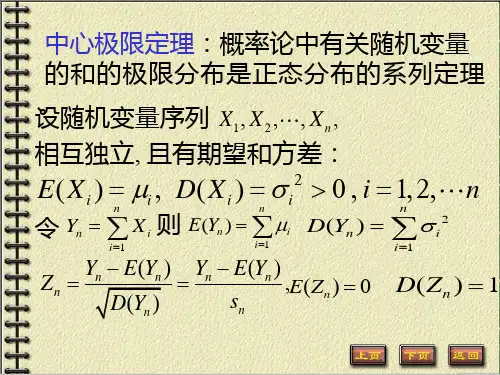
测度论基础与高等概率论21章中心极限定理中心极限定理是概率论中一组重要的定理，用于研究随机变量序列的极限分布。

在测度论基础与高等概率论的21章，涉及到中心极限定理的相关内容，以下是一些相关参考内容：1. 弱大数定律：弱大数定律是中心极限定理中的一种形式，它陈述了当独立同分布（i.i.d.）的随机变量序列的方差有限时，序列的算术平均值以概率1收敛到其数学期望。

弱大数定律表明了当样本容量足够大时，随机变量序列的平均值在概率上趋近于其数学期望。

2. 中心极限定理的基本思想：中心极限定理的基本思想是指出，当独立随机变量的和在适当缩放后对于任意给定的实数都收敛到标准正态分布。

中心极限定理提供了一种将原始数据与正态分布联系起来的方法。

3. 林德伯格中心极限定理：林德伯格中心极限定理是中心极限定理的一种形式，它陈述了当随机变量来自于任何分布（不一定是独立同分布的）且具有有限的均值和方差时，它们的标准化和服从于标准正态分布。

林德伯格中心极限定理是中心极限定理的一般化，适用范围更广。

4. 切比雪夫不等式：切比雪夫不等式是中心极限定理中的一种工具，它提供了一种估计随机变量与其数学期望之间差距的方法。

切比雪夫不等式指出，对于任意正数ε，当随机变量的方差有限时，不等式P(|X-μ|≥ε)≤σ²/ε²成立，其中X是随机变量，μ是其数学期望，σ是其标准差。

5. 中心极限定理在统计推断和假设检验中的应用：中心极限定理在统计推断和假设检验中具有重要应用。

它可以用来进行参数估计、构造置信区间和进行假设检验。

基于中心极限定理，可以构造统计量，并根据标准正态分布来计算容易估算的概率。

综上所述，中心极限定理是测度论基础与高等概率论中的一个重要内容。

它提供了在独立随机变量序列的极限分布研究中的有力工具，深刻揭示了随机现象背后的规律性。

此外，中心极限定理具有广泛的应用，可以用于统计推断和假设检验等领域，为实际问题的分析和解决提供了有力的数学工具。