旋风分离器气固两相流数值模拟

discussion of the near wall treatment and simply standard wall approach is utilized.However main purpose of this tutorial is to show how to relatively easy create structured mesh for the geometry which automatic mesh generator are not able to handle such meshes.One can try to build geometry with different heater alignments and observe how that influence,theflow,pressure drop,and temperature profile at the outlet of the heater.0.2Cyclone.In many industrial processes emerge a need of cleaning gases from dispersed inert particles suspended within gas(eg.removal offlying ash fromflue gases in industrial coalfired boilers).Easiest and most commonly used method of separation takes advantage of gravitation forces.Device which work on this basis is a cyclone.With this tutorial we build simple cyclone geometry,mesh it, and run Fluent simulations.Instead offlue gases we will use air stream polluted with ash.Data for boundary conditions are given in Table2.airflow0.27m3n/sairflow temperature500Cash massflux0.001kg/smin.particle diameter1µmmax.particle diameter300µmmean particle diameter150µmspread parameter 2.8ash density2100kg/m3Table2:Cyclone running parameterFigure9shows cyclone dimensions.Geometry of the cyclone is build in Gambit using volume primitives.Figure10shows all volumes used to build the cyclone which are connected using boolean operations.0.2.1Building geometryProcedure of building the cyclone geometry is very simple.First we create and move in the right position volume primitives presented in Figure10.Next boolean summation and subtraction is used to unite all primitives in order to create one volume representing a cyclone.See below listing of the geometry cre-ation procedure.Listing shows order of operations to be carried out in Gambit. Geometry→Volume→Create Volume→CylinderEnter Height=0.5,Radius1=0.3,Radius2=0.3press Apply11Figure9:Cyclone dimensions. Geometry→Volume→Create Volume→FrustumEnter Height=1.0,Radius1=0.3,Radius2=0.3,Radius3=0.1 press ApplyGeometry→Volume→Move/Copy/AlignSelect with the mouse created frustum:Pick Volume2Check Move,TranslateEnter X=0,Y=0,Z=0.5press ApplyGeometry→Volume→Create Volume→CylinderEnter Height=0.05,Radius1=0.1,Radius2=0.112Figure10:Volume primitives for Cyclone.press ApplyGeometry→Volume→Move/Copy/AlignSelect with the mouse created cylinder:Pick Volume3 Check Move,TranslateEnter X=0,Y=0,Z=1.5press ApplyGeometry→Volume→Create Volume→CylinderEnter Height=0.15,Radius1=0.2,Radius2=0.2press ApplyGeometry→Volume→Move/Copy/AlignSelect with the mouse created cylinder:Pick Volume413Check Move,TranslateEnter X=0,Y=0,Z=1.55press ApplyGeometry→Volume→Create Volume→CylinderEnter:Height=0.8,Radius1=0.1,Radius2=0.1press ApplyGeometry→Volume→Move/Copy/AlignSelect with the mouse created cylinder:Pick Volume5Check Move,TranslateEnter X=0,Y=0,Z=-0.2press ApplyGeometry→Volume→Create Volume→BrickEnter Width=0.2,Depth=0.7,Height=0.2press ApplyGeometry→Volume→Move/Copy/AlignSelect with the mouse created cylinder:Pick Volume6Check Move,TranslateEnter X=0.2,Y=0.35,Z=0.1press ApplyGeometry→Volume→Boolean Operations→UniteSelect with the mouse all the volumes except last created(Volume6):Pick Vol-ume1,Volume2,Volume3,Volume4,Volume5press ApplyGeometry→Volume→Boolean Operations→SubtractSelect with the mouse the volumes which is result of last operation:Volume Volume1Select with the mouse remaining volume:Subtract Volume Volume5Check Retain under Subtract Volumepress ApplyGeometry→Face→Connect/Disconnect Faces→ConnectSelect with the mouse faces aligned between volumes,only this which are at the cover of small cylinder,seefigure11.This operation is needed to force continuum between volumes.It results in deleting one of the face which are aligned at the same position.After operation two volumes are linked by one face forcing later the same mesh to be generated for both volumes at that face. Not connected faces will be by default treated as wall.In our case,side cylinder face of the Volume5will be a wall.press Apply after making selection14Figure11:Faces to be selected for Face Connect oparation.0.2.2Setting boundary condition typesIn order to indicate inlet and outlet of the cyclone we need to specify boundary condition types in Gambit.Additionally ash hopper has to be marked as sepa-rate wall,this is required for dispersed phase modelling.See listing of boundary types setting below.Zones→Specify Boundary TypesCheck(Add)Enter,Name:inSelect Type VELOCITY INLETPick Entity:Faces,face representing inlet to the cyclone,see Figure12press ApplyZones→Specify Boundary TypesCheck(Add)Enter,Name:outSelect Type OUTFLOWPick Entity:Faces,face representing outlet from the cyclone,see Figure12 press Apply15Zones →Specify Boundary Types Check (Add )Enter,Name:ash Select Type WALLPick Entity :Faces ,faces creating ash hopper,see Figure 12pressApplyFigure 12:Boundary condition types.0.2.3Meshing geometryGeneration of appropriate mesh for cyclone geometry is not a trivial task.The flow inside a cyclone is fully 3dimensional and complex.Proper simulation of such flow require careful treatment of the mesh.Since this exercise is only to show possibilities of Fluent and we rather would like to show general procedure of simulating cyclone operation automatic mesh generator will be used.It is advised never to use shown here mesh for simulations of real object.See below16procedure for meshing cyclone geometry.Mesh→FacePick Faces,select all the facesSelect Elements:TriSelect Type:PaveCheck Spacing:ApplyEnter Interval size0.05Press ApplyMesh→VolumePick Volumes,select all the volumesSelect Elements:Tet/HybridSelect Type:TgridUncheck Spacing:ApplyPress ApplyFinal mesh should contain around20000cells.The last task to perform in Gambit is to export generated mesh to thefile.File→Export→MeshPress Browse to select destination folder.Enter name of thefile,extension will be given by default.Press Accept0.2.4Setting Fluent parametersHerewith procedure of setting up cyclone simulations in Fluent.Read meshfile(meshfiles have extension˙msh)created in previous section. File→Read→Case...Define solver settings as default.Define→Models→Solver...Set turbulence modellDefine→Models→Viscous...Select k− RNG turbulence model with option Swirl Dominated FlowIn the Discrete Phase Model panel change Maximum Number of Steps to10000 Set InjectionsSelect Injection Type→surfaceSelect Release From Surfaces→in(in is an inlet face)Select Material→ashSelect Diameter Distribution→rosin-rammler-logarithmicSelect tab Point PropertiesEnter Total Flow Rate(kg/s)equal to0.001Enter Min.Diameter(m)equal to1e-6Enter Max.Diameter(m)equal to300e-617Enter Mean Diameter(m)equal to150e-6Enter Spread Parameter equal to2.8Enter Number of Diameters equal to15Select tab Turbulent DispersionFrom Stochastic Tracking select Discrete Random Walk ModelEnter Number of Tries equal to5Accept settings pressing OKDefine material properties Define→Materials...Change density for airEnter Density(kg/m3)equal to1.094Confirm changes pressing Change CreateChange density for inert-particle ashEnter Density(kg/m3)equal to2100Confirm changes pressing Change CreateDefine operating condition Define→Operating Conditions...Select GravityEnter gravitation acceleration Z(m/s2)equal to9.81Accept settings pressing OKDefine boundary condition Define→Boundary Conditions...Select Zone→in,press SetEnter Velocity Magnitude(m/s)equal to7.98Select Turbulence Specification Method→Intensity and Hydraulic Diameter Enter Hydraulic Diameter(m)equal to0.2Accept settings pressing OKSelect Zone→ash,press SetSelect tab DPMUnder Discrete Phase Model Condition select Boundary Cond.Type→trap Accept settings pressing OKSelect Zone→wall,press SetSelect tab DPMUnder Discrete Phase Reflection Condition select Normal→constantEnter value equal to0.8Under Discrete Phase Reflection Condition select Tangent→constantEnter value equal to0.8Accept settings pressing OKClose Boundary Condition panelset up solver parameters Solve→Controls→Solution...From Discretization select Momentum→Second Order UpwindFrom Discretization select Turbulent Kinetic Energy→Second Order Upwind From Discretization select Turbulent Dissipation Rate→Second Order Upwind Accept settings pressing OKInitialize solution Solve→Initialize→Initialize...Press Init and close Solution Initialization panelSet solution monitoring option Solve→Monitors→Residual...Under Option select PlotFor Residual→continuity→Convergence Criterion enter value equal to10e-918Accept settings pressing OKsave Fluent settings parameter in casefile(casefiles have extension.cas)File →Write→Case...,enterfile name and accept settings pressing OK0.2.5Performing calculationsHerewith we assume that Fluent is open and casefile with cyclone is read. Type in Fluent command window it100,(this command executes100iterations) Observe in Fluent result window residuals of the solved equationsCreating planes for extracting calculated variablesRunning simulations on3D domain we do not have direct access to solved vari-able inside the ing Fluent post processing tools we can display only variables on the external boundary of the domain.In order to access variable inside the domain internal lines or planes needs to be created.The best of the flow visualization is to look at variables(velocity,pressurefield)on the plane inside the domain.Planes can be placed at arbitral position selected by the user.From the number of methods of defining planes position available in Flu-ent we suggest to use3points method described below.Just in case we do not remember size of the domain geometry and its placement in the cartesian system we can display cartesian coordinates on the external boundaries of the domain geometry(see listing below).Select Display→Contours...From Option select FilledFrom Contours of select Grid→X-coordinateFrom Surfaces select wallPress DisplayObserve in Fluent result window boundary of the domain colored by X cartesian coordinateRepeat operation for Contours of→Y-coordinate and Z-coordinateThe cyclone axis is aligned with Z axis and crossing X=0and Y=0cartesian coordinates.Now we create plane crossing cyclone for Y=0.Select Surface→Plane...From Points enter,x0(m)=1,x1(m)=0,x2(m)=0y0(m)=0,y1(m)=0,y2(m)=0z0(m)=0,z1(m)=0,z2(m)=1(exact coordinates are not important,points can not be aligned,and in our case all y variables must be equal to0)19For New Surface Name enter desired name of the surface and press Create Close Plane Surface panel pressing CloseYou can repeat procedure above to create more planes in the arbitral positions inside analyzed domain.You can see created planes by displaying them in the Fluent result window.Select Display→Grid...Select All from Edge TypeFrom Surface select name of the creates palnePress DisplayDisplaying Fluent variables on created planesFluent provide extremely powerful post processing tool.It allows to display on the screen all calculated variables and number of predefined derivatives of these variables.Here we show general procedure of displaying variables on created planes.Select Display→Contours...From Option select FilledFrom Contours of,select Pressure...→Static PressureFrom Surfaces select plane created in previous stepPress DisplayObserve in Fluent result window plane colored by static pressurefield,one can see that the boundary of the domain are not visible,From Option select Draw Grid panel Grid Display pop upsFrom Edge Type select Feature,and from Surfaces select domain boundary you want to displayPress Display,now,when displaying contours of variables simultaneously domain boundary wireframe will be displayedFrom Contours of,select Velocity...→Velocity MagnitudePress DisplayObserve in Fluent result window plane colored by velocity magnitudefield,and the boundary of the domainSimulating ashflying inside a cyclone-particle trackingIn most of the cases mass load of the inert particles is small comparing to trans-port gas.If heat transfer between phases in not involved particle can be,without considerable error,traced within a gas phase in the frame of postprocessing.It means thatfirst we simulatefluidflow of a gas phase.When convergence for continues phase is reached inert particle representing ash are traced employing20Lagrangian model.See below for executing tracing procedure.Select Display→Particle Tracks...From Option activate Draw Grid in order to see boundary of the domain(see section above for explanation)From Release from Injections select injection-0,(name can be different)Select Track Single Particle Stream,(number of particle traced usually exceed thousands and tracking procedure in lengthly even on fast computers,in orderto make this faster and be able to see particle paths on the screen we select this option→particle will be send only from one face at the inlet)Press Display,(Fluent starts tracing procedure,afterfinishing displays particle paths in results window.In the main Fluent window report of the tracing procedure is printed.Report shows how many particles have been traced,trapped,escaped,aborted and in-complete,evaporated for inert particle is meaningless.Trapped are particle col-lected in the ash hopper.Escaped are these which left the cyclone through the outlet.Aborted are not traced by the solver due to numerical error.Incomplete are these for which Max.Number of Steps was not enough to complete tracing. See section0.2.4for changing Max.Number of Steps for particle tracking.) Useful option in particle tracking procedure is summary report.It can helpin assessing efficiency of cyclone which is calculated as ratio of the ash massflux collected inside ash hopper to the ash massflux entering a cyclone.It also informs of the massflux of incomplete traces.The regular report provide only the number of trapped,escaped and incomplete streams which is meaningless in assessing cyclone operation.See procedure below for activating summary report. Within Particle Trucks panel,select Summary from Report TypeDeselect Track Single Particle StreamPress Track,(particle steams will not be displayed in results window)See below example of summary report:number tracked=3300,escaped=419,aborted=0,trapped=2362,evaporated=0,incomplete=519Fate Number Elapsed Time(s)Injection,IndexMin Max Avg Std Dev Min Max ------------------------------------------------------------------------------------------Incomplete519 5.646e-001 4.080e+000 1.130e+000 3.826e-001injection-00injection-0515 Trapped-Zone423627.418e-001 3.770e+000 1.509e+000 3.425e-001injection-0424injection-0203 Escaped-Zone5419 3.792e-001 3.530e+000 1.003e+000 5.647e-001injection-048injection-0275 (*)-Mass Transfer Summary-(*)Fate Mass Flow(kg/s)Initial Final Change----------------------------------Incomplete 2.897e-008 2.897e-0080.000e+000Trapped-Zone49.996e-0049.996e-0040.000e+000Escaped-Zone5 3.562e-007 3.562e-0070.000e+000The most interesting is Mass Transfer Summary which shows massfluxes of Incomplete,Trapped and Escaped particle streams.General report shows only number of incomplete,trapped and escaped particle stream.Sometimes even21large number of escaped particle streams not impose low cyclone efficiency, because these streams could be low diameter particle streams.Hence in order to asses cyclone efficiency massfluxes of trapped and escaped particle streams needs to be compared.Escaped particle stream number indicate how many trace of the particle streams has not been completed.There are neither trapped nor escaped and traced has beenfinished inside domain.If number and massflux of incomplete stream is large we need to increase Max.Number of Steps under Discrete Phase Model panel opened from Define menu.22。

旋风分离器气固两相流数值模拟及性能分析共3篇旋风分离器气固两相流数值模拟及性能分析1旋风分离器气固两相流数值模拟及性能分析旋风分离器是一种广泛应用于化工、环保、电力等领域的气固分离设备，其利用离心力将气固两相流中的颗粒物分离出来，一般被用作除尘和粉尘回收设备。

本文将介绍旋风分离器的气固两相流数值模拟及性能分析。

气固两相流是指气体与固体颗粒混合物流动的状态。

旋风分离器中的气固两相流在进入设备后，经过导流装置后便会进入旋风筒，此时气固两相流呈螺旋上升流动状态，颗粒物受到离心力的作用被抛向旋风筒壁，而气体则从旋风筒顶部中心脱离，从出口排放。

因此，旋风分离器气固两相流的流体物理特性显得尤为重要。

本文采用计算流体力学（Computational Fluid Dynamics，CFD）方法对旋风分离器气固两相流进行数值模拟。

对于气体流动部分，采用了二维轴对称的控制方程式，包括连续性方程、动量方程和能量方程，而对于颗粒物流动部分，采用了颗粒物轨迹模型（Particle Tracking Model，PTM）。

在数值模拟过程中，采用了FLUENT软件进行求解，其中的数值算法采用双重电子数法（Electron Electrostatic Force Field，E3F2）。

数值模拟结果显示，在旋风分离器中，气体的流速主要集中在筒壁附近，而在离筒中心较远的地方，则流速较慢，颗粒物则以螺旋线的方式向旋风筒壁移动，并沿着筒壁向下运动。

颗粒物在旋风筒中受到离心力的作用后，其分布状态将随着离心力的变化而变化，最终沉积在筒壁处。

数值模拟结果还表明，旋风分离器的分离效率随着旋风筒直径的增加而增加。

为了验证数值模拟结果的可信度，实验室制作了一个小型旋风分离器进行了实验研究。

实验结果表明，数值模拟与实验结果相比较为一致，通过数值模拟可以较好地描述旋风分离器中气固两相流动的情况并用于性能预测。

综合来看，数值模拟是一种较为有效的旋风分离器气固两相流性能分析方法，可以较好地预测旋风分离器的分离效率和颗粒物的分布状态，为旋风分离器的设计和优化提供了有力支持综上所述，本文利用数值模拟方法和实验研究相结合的方式，对旋风分离器的气固两相流动性能进行了分析。

旋风分离器气固流动特性数值模拟研究
钱玉宝;郭旭涛;邱腾煌
【期刊名称】《轻金属》
【年(卷),期】2024()1
【摘要】为探究旋风分离器流场特性与分离特征,在气固两相流理论基础上,建立旋风分离器结构模型,通过CFD数值模拟软件对分离器的流场进行仿真计算,研究了气相速度场和压力场分布情况,考察各项参数对分离性能的影响。

进行方案优选,在圆柱段长度430 mm、下锥段长度790 mm、溢流管插入深度140 mm、溢流口直径80 mm时分离器分离效率达到最优值。

通过线性回归与多元逐步回归法推导得出分离效率与参数间的关系表达式,对分离器结构改进具有重要的参考价值。

【总页数】8页(P18-24)
【作者】钱玉宝;郭旭涛;邱腾煌
【作者单位】长江大学机械工程学院;湖北省油气钻完井工具工程技术研究中心;中石化石油机械股份有限公司
【正文语种】中文
【中图分类】TF821
【相关文献】
1.循环流化床锅炉旋风分离器内气固两相流动的数值模拟
2.多喷嘴射流式分离器内气固流动特性的数值模拟
3.旋风分离器内气固两相流动特性的模拟研究
4.循环流化床锅炉旋风分离器内气固两相流动的数值模拟
因版权原因，仅展示原文概要，查看原文内容请购买。

旋风分离器在工业上的应用已有百年多的历史。

它是利用气固两相流的旋转，将固体颗粒从气流中分离出来的一种干式气-固分离装置[1]。

与其它气固分离设备相比，具有结构简单、设备紧凑、性能稳定和分离效率高等特点。

广泛应用于石油、化工、冶金、建筑、矿山、机械和环保等工业部门。

由于旋风分离器内部流动非常复杂，用试验或者解析的方法研究分离器内部的流动状况比较困难。

近年来，随着计算机硬件及CFD(计算流体动力学)技术的不断进步[2,3]，数值方法成为研究旋风分离器的一种重要手段。

通过对旋风分离器内气固两相进行数值模拟，揭示旋风分离器内部流场，为优化旋风分离器的结构提供思路，也为进一步提高分离性能奠定基础。

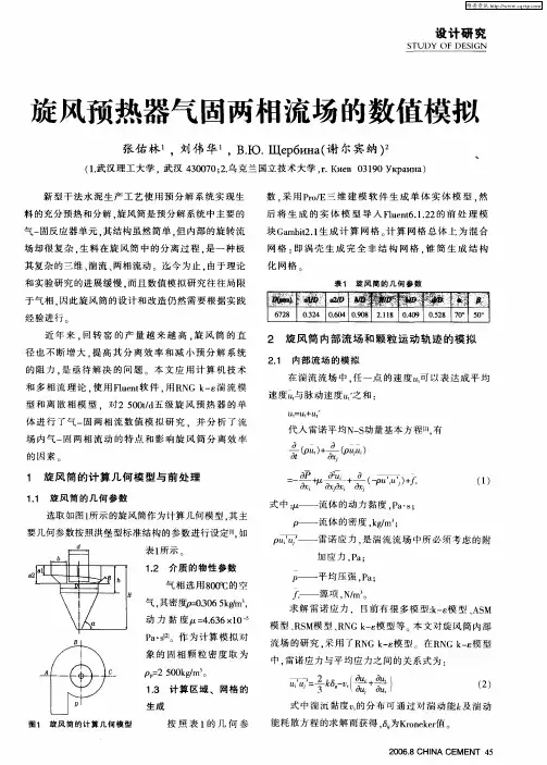
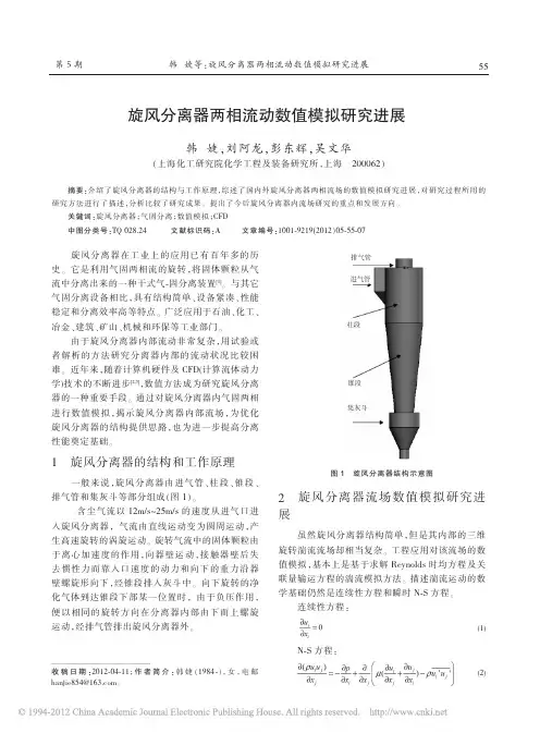
1旋风分离器的结构和工作原理一般来说，旋风分离器由进气管、柱段、锥段、排气管和集灰斗等部分组成（图1）。

含尘气流以12m/s ～25m/s 的速度从进气口进入旋风分离器，气流由直线运动变为圆周运动，产生高速旋转的涡旋运动。

旋转气流中的固体颗粒由于离心加速度的作用，向器壁运动，接触器壁后失去惯性力而靠入口速度的动力和向下的重力沿器壁螺旋形向下，经锥段排入灰斗中。

向下旋转的净化气体到达锥段下部某一位置时，由于负压作用，便以相同的旋转方向在分离器内部由下而上螺旋运动，经排气管排出旋风分离器外。

2旋风分离器流场数值模拟研究进展虽然旋风分离器结构简单，但是其内部的三维旋转湍流流场却相当复杂。

工程应用对该流场的数值模拟，基本上是基于求解Reynolds 时均方程及关联量输运方程的湍流模拟方法。

描述湍流运动的数学基础仍然是连续性方程和瞬时N -S 方程。

连续性方程：N -S 方程：收稿日期：2012-04-11；作者简介：韩婕（1984-），女，电邮hanjie854@ 。

旋风分离器两相流动数值模拟研究进展韩婕，刘阿龙，彭东辉，吴文华（上海化工研究院化学工程及装备研究所，上海200062）摘要：介绍了旋风分离器的结构与工作原理，综述了国内外旋风分离器两相流场的数值模拟研究进展，对研究过程所用的研究方法进行了描述，分析比较了研究成果。

基于CFD的循环流化床旋风分离器数值模拟
循环流化床旋风分离器是广泛应用于化学反应、热处理和废气处理等领域的重要设备。

该设备将固体物料以流化床形式进行循环，通过旋风分离器分离气固两相，实现了在化工、环保工程等领域的重要应用。

为了在设计和改进该设备时准确预测流动和分离的特性，数值模拟成为一种有效的方法。

基于CFD的循环流化床旋风分离器数值模拟已经成为一种快速、准确预测流动和分离过程的工具。

CFD数值模拟的过程首先需要准确建立数值模型，进行网格划分和边界条件设定。

然后利用计算机运算能力，通过数值模拟解决数学模型得到流动和分离的过程。

最后，通过数值模拟的结果，可以解决实际设计和改进的问题。

在这个过程中，需要确定正确的物理模型、适当的边界条件和网格密度以及求解方法等。

对于循环流化床旋风分离器的数值模拟，需要考虑以下几个因素。

首先，需要考虑气固两相之间的相互作用。

流化床内气固两相的运动应当由玻意耳数学模型来描述，同时应当将压降等现象考虑在内。

其次，流化床内的颗粒运动也应当考虑，因此某些模拟需采用多相流模型。

此外，旋风分离器中气相的旋转和离心效应都应当加以考虑。

基于CFD的循环流化床旋风分离器数值模拟具有许多优点。

其能够快速准确地预测流动和分离过程，可以帮助研究人员了
解设备内部的运动规律，进而优化设计、提高设备效率。

此外，该方法还可以帮助研究人员验证实验数据，并减少试验成本和时间。

因此CFD模型应用于该设备的设计和改进中，可以提
高效率，节约成本，同时优化产品质量和制造n优化生产成果。

硕士学位论文旋风分离器气固两相流数值模拟及性能分析NUMERICAL SIMULATION AND PERFORMANCE ANALYSIS OF GAS-SOLID TWO PHASE FLOW IN CYCLONE SEPARATOR汪 林哈尔滨工业大学2007年7月国内图书分类号：TU834.6国际图书分类号：626工学硕士学位论文旋风分离器气固两相流数值模拟及性能分析硕士研究生：汪林导师：朱蒙生 副教授申请学位：工学硕士学科、专业：水力学及河流动力学所在单位：市政环境工程学院答辩日期：2007年7月授予学位单位：哈尔滨工业大学Classified Index: TU834.6U.D.C: 626Dissertation for the Master Degree in EngineeringNUMERICAL SIMULATION AND PERFORMANCE ANALYSIS OF GAS-SOLID TWO PHASE FLOW INCYCLONE SEPARATORCandidate:Supervisor:Academic Degree Applied for: Speciality:Affiliation:Date of Defence:Degree-Conferring-Institution:Wang LinAssociate Prof. Zhu Mengsheng Master of Engineering Hydraulics and River Dynamics School of Municipal & Environmental Engineering July, 2007Harbin Institute of Technology摘要摘要近年来，随着人们环境保护意识的加强，以旋风分离器为代表的各类除尘设备已经成为防治大气污染的主力军，在消除大气污染、保障人类健康及生态环境方面发挥着重要作用。

旋风分离器的气固两相特性研究与数值模拟摘要旋风分离器是一种利用气固两相流体的旋转运动使固体颗粒在离心力的作用下从气流中分离出来的设备。

它具有结构简单，维护方便，耐高温、高压，造价低等优点，在环保、粉体、石油、化工、冶金、材料等许多领域有着广泛的应用，使得旋风分离器的研究越来越受到重视。

旋风分离器的应用已经有很长一段历史了，由于旋风分离器中的含尘气流属于三维强旋转湍流，伴随着两相分离运动，而且涉及到气固两相相互作用以及凝聚、吸附和静电等许多复杂物理现象，使得理论研究遇到很大困难，理论进展缓慢。

传统的设计是依据己知的操作条件和所需的性能指标，凭借经验先选定旋风分离器的结构形式及尺寸，然后通过半经验公式计算出旋风分离器的效率及压降，再根据计算结果修改尺寸。

设计过程具有很大的盲目性。

本文利用计算流体力学商业软件FLUENT对旋风分离器进行了数值模拟。

在选择了合适的数值模拟方案后，模拟研究了多种情况下的气相速度场、压力场、颗粒运动轨迹、颗粒分级效率、旋风分离器总分离效率等参数。

通过本文大量的数值模拟研究，主要得到了以下这些结论：1) 通过研究确立了一套最适合旋风分离器内部气相流场的数值计算方法：湍流模型采用雷诺应力模型；差分格式采用QUICK格式；压力梯度项插补格式采用PRESTO格式；计算方法采用SIMPLEC算法。

2) 旋风分离器内的气相主流是双层旋转流，外部是回转向下的外旋转流，而中心是向上旋转的内旋流，且两者的旋转方向相同。

切向速度分布呈现了组合涡的特点，中心区域为强制涡，外部区域为准自由涡。

3) 旋风分离器中旋涡具有不稳定性，它会引起涡核尾部或端部附着在旋风分离器下部壁面并旋转摆动，使得返混现象变严重，同时还会引起结垢现象。

4) 旋风分离器内静压在径向上随着径向尺寸的减小而降低；动压在强制涡和准自由涡的分界面CS处最大。

分离器总压降包括静压降和动压降两部分。

5) 旋风分离器中的颗粒运动很复杂，总的来说，从入口外侧和下方入射的颗粒分别较从内侧和上方入射的颗粒更容易分离。