实验二 MATLAB基础知识(二)

实验一 MATLAB入门（1）1.实验目的：（1）了解MATLAB的体系结构与特点，熟悉其集成开发环境。

（2）熟悉MATLAB界面窗口的功能和使用方法。

（3）熟悉MATLAB的帮助系统及使用方法。

（4）了解MATLAB的的数据类型、基本形式和数组的产生方法。

（5）掌握MATLAB基本的数学运算操作。

2.实验原理（1）MATLAB简介MATLAB是美国MathWorks公司开发的高性能的科学与工程计算软件。

它在数值计算、自动控制、信号处理、神经网络、优化计算、小波分析、图像处理等领域有着广泛的用途。

近年来， MATLAB在国内高等院校、科研院所的应用逐渐普及，成为广大科研、工程技术人员必备的工具之一。

MATLAB具有矩阵和数组运算方便、编程效率极高、易学易用、可扩充性强和移植性好等优点，俗称为“草稿纸式的科学计算语言”。

它把工程技术人员从繁琐的程序代码编写工作中解放出来，可以快速地验证自己的模型和算法。

经过几十年的扩充和完善,MATLAB已经发展成为集科学计算、可视化和编程于一体的高性能的科学计算语言和软件开发环境，整套软件由MATLAB开发环境、MATLAB语言、MATLAB数学函数库、MATLAB图形处理系统和MATLAB应用程序接口（API）等五大部分组成。

MATLAB的主要特点包括强大的计算能力（尤其是矩阵计算能力）、方便的绘图功能及仿真能力、极高的编程效率。

另外，MATLAB还附带了大量的专用工具箱，用于解决各种特定领域的问题。

通过学习软件的基本操作及其编程方法，体会和逐步掌握它在矩阵运算、信号处理等方面的功能及其具体应用。

通过本课程实验的学习，要求学生初步掌握MATLAB的使用方法，初步掌握M文件的编写和运行方法，初步将MATLAB运用于数字信号处理中。

循序渐进地培养学生运用所学知识分析和解决问题的能力。

（2）MATLAB的工作界面（Desktop）与操作MATLAB 安装成功后，第一次启动时，主界面如下图（不同版本可能有差异）所示：其中① 是命令窗口（Command Window ），是MATLAB 的主窗口，默认位于MATLAB界面的右侧，用于输入命令、运行命令并显示运行结果。

grid on %在所画出的图形坐标中加入栅格
绘制图形如下
50
10
1
0.8
40
10
0.6
0.4
30
10
0.2
0
1020
-0.2
-0.4
1010
-0.6
-0.8
0
10
-1
-2
0
2
-2
0
2
10
10
10
10
10
10
如果在图中不加栅格
程序如下：
clear x=logspace(-1,2);%在10^(-1)到10^2之间产生50个 对数等分的行向量 subplot(121); loglog(x,10*exp(x),'-p') subplot(122); semilogx(x,cos(10.^x))
（2）plot(x,y)： 基本格式，x和y可为向量或矩阵. 1. 如果x，y是同维向量，以x元素为横坐标，以y元素 为纵坐标绘图. 2. 如果x是向量，y是有一维与x元素数量相等的矩阵， 则以x为共同横坐标， y元素为纵坐标绘图，曲线数目 为y的另一维数. 3. 如果x，y是同维矩阵，则按列以x，y对应列元素为 横、纵坐标绘图，曲线数目等于矩阵列数.
y=2*exp(-0.5*x).*cos(4*pi*x);
2
plot(x,y)
1.5
1
0.5
0
-0.5
-1
-1.5
-2
0
1
2
3
4
5
6
7
例4 绘制曲线
t=(0:0.1:2*pi);
x=t.*sin(3*t);
y=t.*sin(t).*sin(t);

a=[1 2 1;2 2 1;2 1 2]; b=[1;2;3]; a/b %矩阵右除
运行程序，得到结果：
??? Error using ==> mrdivide Matrix dimensions must agree.
重新输入语句
a\b
%矩阵左除 ans = 1.0000 -0.3333 0.6667
运行程序，得到结果：
c= 0 0 1 1 1 0
说明 对于复数运算，“= =”与“～ =”运算，既比较实部， 又比较虚部。而其他运算仅比较实部。关系运算同样也可用于 常量与矩阵的比较，在这种情况下，该常量与矩阵的每一个元 素进行比较，其结果是一个与矩阵同维数的0、1矩阵。
逻辑操作符
逻辑操作符 说 明 相对应函数
-0.1667 0 0
（3）矩阵特征值运算
矩阵条件数cond( ) 矩阵的秩rank() 矩阵特征值eig ( )
矩阵范数norm( ) 矩阵的迹trace ( ) 矩阵奇异值svd ( )
例2-7 分别计算矩阵a的有关特征参数。输入以下 MATLAB语句
a=[1 2 3;4 5 6;7 8 0] [cond(a),norm(a),rank(a)]
2.MATLAB工作环境
图形窗口“Figure”
M文件窗口
3．MATLAB的M文件
所谓M文件，就是用户把要实现的命令写在一个 以.m为扩展名的文件中
M文件有两种格式（统称为M文件） 函数式M文件 程序式M文件 程序式M文件用于把很多需要在命令窗口输入的命 令放在一起，就是命令的简单叠加 函数式M文件用于把重复的程序段封装成函数供用 户调用。
&
|
逻辑与
逻辑或
and(a,b)

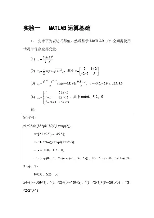
实验一 MATLAB 运算基础1、 先求下列表达式得值，然后显示MATLAB 工作空间得使用情况并保存全部变量。

(1) 0122sin 851z e =+(2) 21ln(2z x =+，其中2120.455i x +⎡⎤=⎢⎥-⎣⎦ (3) 0.30.330.3sin(0.3)ln , 3.0, 2.9,,2.9,3.022a a e e a z a a --+=++=--L (4) 2242011122123t t z t t t t t ⎧≤<⎪=-≤<⎨⎪-+≤<⎩，其中t =0:0、5:2、5 解：4、 完成下列操作：(1) 求[100,999]之间能被21整除得数得个数。

(2) 建立一个字符串向量，删除其中得大写字母。

解：(1) 结果：(2)、 建立一个字符串向量 例如：ch='ABC123d4e56Fg9';则要求结果就是：实验二 MATLAB 矩阵分析与处理1、 设有分块矩阵33322322E R A O S ⨯⨯⨯⨯⎡⎤=⎢⎥⎣⎦，其中E 、R 、O 、S 分别为单位矩阵、随机矩阵、零矩阵与对角阵，试通过数值计算验证22E R RS A OS +⎡⎤=⎢⎥⎣⎦。

解: M 文件如下；5、 下面就是一个线性方程组：1231112340.951110.673450.52111456x x x ⎡⎤⎢⎥⎡⎤⎡⎤⎢⎥⎢⎥⎢⎥⎢⎥=⎢⎥⎢⎥⎢⎥⎢⎥⎢⎥⎢⎥⎣⎦⎣⎦⎢⎥⎢⎥⎣⎦(1) 求方程得解。

(2) 将方程右边向量元素b 3改为0、53再求解，并比较b 3得变化与解得相对变化。

(3) 计算系数矩阵A 得条件数并分析结论。

解： M 文件如下：实验三 选择结构程序设计1、 求分段函数得值。

2226035605231x x x x y x x x x x x x ⎧+-<≠-⎪=-+≤<≠≠⎨⎪--⎩且且及其他用if 语句实现，分别输出x=-5、0,-3、0,1、0,2、0,2、5,3、0,5、0时得y 值。

实验二、MA TLAB运算基础一、实验目的掌握MA TLAB各种表达式的书写规则及常用函数的使用。

掌握MA TLAB中字符串、元胞数组和结构的常用函数的使用。

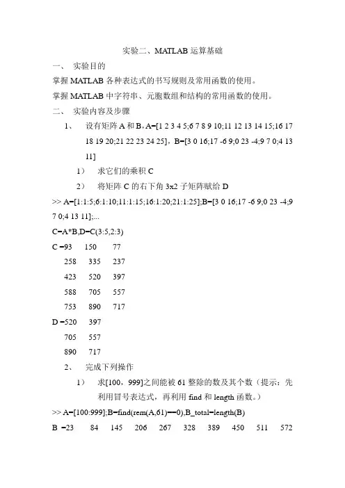
二、实验内容及步骤1、设有矩阵A和B，A=[1 2 3 4 5;6 7 8 9 10;11 12 13 14 15;16 1718 19 20;21 22 23 24 25]，B=[3 0 16;17 -6 9;0 23 -4;9 7 0;4 1311]1）求它们的乘积C2）将矩阵C的右下角3x2子矩阵赋给D>> A=[1:1:5;6:1:10;11:1:15;16:1:20;21:1:25];B=[3 0 16;17 -6 9;0 23 -4;9 7 0;4 13 11];...C=A*B,D=C(3:5,2:3)C =93 150 77258 335 237423 520 397588 705 557753 890 717D =520 397705 557890 7172、完成下列操作1）求[100，999]之间能被61整除的数及其个数（提示：先利用冒号表达式，再利用find和length函数。

）>> A=[100:999];B=find(rem(A,61)==0),B_total=length(B)B =23 84 145 206 267 328 389 450 511 572633 694 755 816 877B_total =152）建立一个字符串向量，删除其中的大写字母（提示：利用find函数和空矩阵。

）>> a=['MA TLAB is important'], b=abs(a); c=find(b<=90 & b>=65) , a(c)=[],a =MA TLAB is importantc = 1 2 3 4 5 6a =is important⑶已知A=[23 10 -78 0；41 -45 65 5；32 5 0 32；6 -5492 14]，取出其前3行构成矩阵B，其前两列构成矩阵C，其左下角3x2子矩阵构成矩阵D，B与C的乘积构成矩阵E，分别求E<D、E&D、E|D、~E|~D。

x,y变化范围均为 [0 2π]。
3. 三维图形
• 三、视点
➢view(az,el)-------------设置观察点方向
az为方位角，el为仰角。 • 方位角为视点位置在XY平面上的投影与X轴形成的角度，
正值表示逆时针，负值表示顺时针。 • 仰角为XY平面的上仰或下俯角，正值表示视点在XY平
面上方，负值表示视点在XY平面下方。
figure grid gtext hold subplot text title xlabel ylabel
创建图形窗口 放置坐标网格线 用鼠标放置文本 保持当前图形窗口内容 创建子图 放置文本 放置图形标题 放置X轴坐标标记 放置Y轴坐标标记
3. 三维图形 • 一、 plot3函数
• 将二维函数plot的功能扩展到三维空间，绘制三维图形。 • 函数格式：plot3(x1,y1,z1,c1,x2,y2,z2,c2,…)
theta=[0:0.01:2*pi];
rho=sin(2*theta).*cos(2*theta);
polar(theta,rho); 绘制极坐标图命令
title('polar plot');
例9、程序：
theta=linspace(0, 2*pi);
r=cos(4*theta);
polar(theta, r);
所组成的画面。
4. 动画设计
• 【例14】 播放一个不断变化的眼球程序段。
• m=moviein(20); 建立一个20个列向量组成的矩阵
• for j=1:20
•
plot(fft(eye(j+10))) %绘制出每一幅眼球图并保存到m矩阵中
• m(:,j)=getframe;

佛山科学技术学院《MATLAB教程第二章实训》报告专业姓名成绩班级学号日期一、目的1.学习matlab的数据类型2.矩阵和数组的算术运算3.字符串4.时间和日期5.结构体和元胞数组6.多维数组7.逻辑运算和关系运算8.数组的信息获取9.多项式二、步骤1.学习matlab的数据类型Matlab R2010a定义了15种基本的数据类型，包括整型、浮点型、字符型和逻辑型等。

用户甚至可以定义自己的数据类型。

Matlab内部的任何数据类型，都是按照数组的形式进行储存和运算的。

数值型包括整数和浮点数，其中整数包括有符号数和无符号数，浮点数包括单精度型和双精度型。

在默认情况下，matlab默认将所有数值都按照双精度浮点数类型来存储和操作。

（1）常数和变量Matlab的常数采用十进制表示，可以用带小数点的形式直接表示，也可以用科学记数法。

数值的表示范围是10^-309-10^309。

变量是数值计算的基本单元。

Matlab与其他的高级语言不同，变量使用是无需先定义，其名称就是第一次合法出现时的名称，因此用起来很便捷。

Matlab的变量命名有一定的规则：a.变量区分字母的大小写。

例如，“a”和“A”是不同的变量。

b.变量名不能超过63个字符，第63个字符后的字符会被忽略。

c.变量名必须以字母开头，变量名的组成可以是任意字母、数字或者下划线，但不能有空格和标点符号。

d.关键字（如if\while等）不能作为变量名。

在matlab中的所有表示符号包括函数名、文件名都是遵循变量名的命名规则。

Matlab中有一些自己的特殊变量，是由系统预先自动定义的，例如：ans——运算结果的默认变量名Pi——圆周率πEps——浮点数的相对误差Inf或inf——无穷大Nan或nan——不定值i或j——i=j=-1^1/2，虚数单位Nargin——函数的输入变量数目Nargout——函数的输出变量数目Realmin——最小的可用正实数Realmax——最大的可用正实数（2）整数和浮点数Matlab提供了8种内置的整数类型，为了在使用时提高运行速度和存储空间，应该尽量使用字节少的数据类型，可以使用类型转换函数将各种整数类型强制相互转换。

MATLAB 实验报告班级:14通信1班 学号:201424124124 姓名:林启铭实验一 MATLAB 运算基础(一)一、实验目的1、掌握建立矩阵的方法。

2、掌握MATLAB 各种表达式的书写规则以及各种运算方法。

二、实验内容1、求下列表达式的值。

（1）20185sin 21ez += MATLAB 代码：z1=2*sin(85*pi/180)/(1+exp(2))%将角度化为弧度z1 =0.2375（2）()x x z ++=1ln 212，其中⎢⎣⎡-=45.02x ⎥⎦⎤+521i (可以分别对矩阵和元素群运算)MATLAB 代码：>> x=[2,1+2i;-0.45,5]x =2.0000 + 0.0000i 1.0000 + 2.0000i-0.4500 + 0.0000i 5.0000 + 0.0000i>> z2=1/2*log(x+sqrt(1+x))z2 =0.6585 + 0.0000i 0.6509 + 0.4013i-0.6162 + 0.0000i 1.0041 + 0.0000i（3）()3.0sin 232.03.0+⋅-=a e e z aa ， 0.3,9.2,8.2,...,8.2,9.2,0.3---=a （结果请用图形表示）（提示：利用冒号表达式生成a 向量；求各点的函数值时用点乘运算）MATLAB 代码：>> a=-3.0:0.1:3.0;%利用冒号表达式生成a 向量，加分号结尾避免大量数据刷屏 >> z3=(exp(0.3.*a)-exp(0.2.*a)).*sin(a+0.3)/2;>> plot(a,z3);%绘制出以a 为自变量，z3为因变量的曲线>>曲线图：2、已知⎢⎢⎢⎣⎡=33412A 65734⎥⎥⎥⎦⎤-7874 和 ⎢⎢⎢⎣⎡=321B 203-⎥⎥⎥⎦⎤-731 求下列表达式的值：（1）A+6*B 和A-B+I （其中I 为单位矩阵）。

实验⼆时域采样与频域采样及MATLAB程序知识讲解实验⼆时域采样与频域采样及M A T L A B程序实验⼆时域采样与频域采样⼀实验⽬的1 掌握时域连续信号经理想采样前后的频谱变化，加深对时域采样定理的理解2 理解频率域采样定理，掌握频率域采样点数的选取原则⼆实验原理1 时域采样定理对模拟信号()a x t 以T 进⾏时域等间隔采样，形成的采样信号的频谱()a X j Ω会以采样⾓频率2()s s TπΩΩ=为周期进⾏周期延拓，公式为： 1??()[()]()a a a s n X j FT x t X j jn T +∞=-∞Ω==Ω-Ω∑ 利⽤计算机计算上式并不容易，下⾯导出另外⼀个公式。

理想采样信号?()a xt 和模拟信号()a x t 之间的关系为： ?()()()a a n xt x t t nT δ+∞=-∞=-∑ 对上式进⾏傅⾥叶变换，得到：()[()()()()j t j t a a a n n X j x t t nT e dt x t t nT e dt δδ+∞+∞+∞+∞-Ω-Ω-∞-∞=-∞=-∞Ω=-=-∑∑??在上式的积分号内只有当t nT =时，才有⾮零值，因此:()()jn T aa n X j x nT e +∞-Ω=-∞Ω=∑上式中，在数值上()()a x nT x n =，再将T ω=Ω代⼊，得到：()()()jn j aa T T n X j x n e X e ωωωω+∞-=Ω=Ω=-∞Ω==∑上式说明采样信号的傅⾥叶变换可⽤相应序列的傅⾥叶变换得到，只要将⾃变量ω⽤T Ω代替即可。

2 频域采样定理对信号()x n 的频谱函数()j X e ω在[0，2π]上等间隔采样N 点，得到 2()()j k NX k X e ωπω== 0,1,2,,1k N =-L则有： ()[()][()]()N N N i x n IDFT X k x n iN R n +∞=-∞==+∑即N 点[()]IDFT X k 得到的序列就是原序列()x n 以N 为周期进⾏周期延拓后的主值序列，因此，频率域采样要使时域不发⽣混叠，则频域采样点数N 必须⼤于等于时域离散信号的长度M （即N M ≥）。

实验二MATLAB语言基础一、实验目的基本掌握MA TLAB向量矩阵数组的生成及基本运算（区分数组运算和矩阵预算）、常用的数学函数。

了解字符串的操作。

二、实验内容（1）向量的生成和运算。

（2）矩阵的创建、引用和运算。

（3）多维数组的创建和运算。

（4）字符创的操作。

三、实验步骤1.向量的生成和运算1）向量的生成<1>、直接输入法<2> 冒号表达式法<3> 函数法：Linspace()是线性等分函数，logspace（）是对数等分函数。

2）向量的运算1>维数相同的行、列向量之间可以相加减，标量可以与向量直接相乘除。

2>向量的点积与叉积运算E1和E2虽然表达式相同，但E1是标量，E2是矩阵。

2.矩阵的创建、引用和运算1)矩阵的创建和引用矩阵是由m*n元素构成的矩形结构，行向量和列向量是矩阵的特殊形式。

1>直接输入法：2>抽取法：包括单下标抽取和全下表抽取两种方式，且两种方式抽取的元素都必须以小括号括起来。

3>函数法：利用ones(m;n)创建全1矩阵，zeros（）创建全0矩阵，eyes（）创建单位矩阵等等。

4>拼接法：纵向拼接横向拼接5>利用拼接函数cat（）repmat（）和变形函数reshape（）>> A1=[1 2 3;9 8 7 ;4 5 6];A2=A1.';>> cat(1,A1,A2) 沿行向拼接ans =1 2 39 8 74 5 61 9 42 8 53 7 6>> cat(2,A1,A2) 沿列向拼接ans =1 2 3 1 9 49 8 7 2 8 54 5 6 3 7 6>> repmat(A1,2,2)ans =1 2 3 1 2 39 8 7 9 8 74 5 6 4 5 61 2 3 1 2 39 8 7 9 8 74 5 6 4 5 6> A=linspace(2,18,9)A =2 4 6 8 10 12 14 16 18 >> reshape(A,3,3)ans =2 8 144 10 166 12 182）矩阵的运算练习（1）用矩阵除法求下列方程组的解x=[x1;x2;x3]>> A=[6 3 4;-2 5 7;8 -1 -3];B=[3;-4;-7];X=A\BX =1.0200-14.00009.7200(2)求矩阵的秩A=[6 3 4;-2 5 7;8 -1 -3];>> rank(A)ans =3[X,lamda]=eig(A)X =0.8013 -0.1094 -0.16060.3638 -0.6564 0.86690.4749 0.7464 -0.4719lamda =9.7326 0 00 -3.2928 00 0 1.5602（3）矩阵的开方>> B=sqrtm(A)B =2.2447 + 0.2706i 0.6974 - 0.1400i 0.9422 - 0.3494i -0.5815 + 1.6244i 2.1005 - 0.8405i 1.7620 - 2.0970i1.9719 - 1.8471i -0.3017 + 0.9557i 0.0236 +2.3845i （4）矩阵的指数与对数：> C=expm(A)C =1.0e+004 *1.0653 0.5415 0.63230.4830 0.2465 0.28760.6316 0.3206 0.3745>> logm(C)ans =6.0000 3.0000 4.0000-2.0000 5.0000 7.00008.0000 -1.0000 -3.0000（6）矩阵的转置D=A'D =6 -2 83 5 -14 7 -3（7）矩阵的提取与翻转：通过各种特定函数如triu（A）、tril（A），diag（A）、flipud （A）、fliplr（A）等等。

matlab2022实验2参考答案报告名称：MATLAB试验二符号计算姓名：学号：专业：班级：MATLAB实验二MATLAB符号计算试验报告说明：1做试验前请先预习，并独立完成试验和试验报告。

2报告解答方式：将MATLAB执行命令和最后运行结果从命令窗口拷贝到每题的题目下面，请将报告解答部分的底纹设置为灰色，以便于批阅。

3在页眉上写清报告名称，学生姓名，学号，专业以及班级。

3报告以Word文档书写。

一目的和要求1熟练掌握MATLAB符号表达式的创建2熟练掌握符号表达式的代数运算3掌握符号表达式的化简和替换4熟练掌握符号微积分5熟练掌握符号方程的求解二试验内容1多项式运算（必做）1.1解方程:f(某)=某^4-10某某^3+34某某^2-50某某+25=0%采用数值方法：>>f=[1-1034-5025];>>root(f)%采用符号计算方法：f1=ym('某^4-10某某^3+34某某^2-50某某+25')olve(f1)1.2求有理分式R=(3某^3+某)(某^3+2)/((某^2+2某-2)(5某^3+2某^2+1))的商多项式和余多项式.a1=[3010];a2=[1002];a=conv(a1,a2);b1=[12-2];b2=[5201];b=conv(b1,b2);[p,r]=deconv(a,b);%注意：ab秩序不可颠倒。

%reidue用于实现多项式的部分分式展开，此处用deconv函数报告名称：MATLAB试验二符号计算姓名：学号：专业：班级：%%此题，有同学程序如下：某1=[3010]，某2=[1002],某3=[12-2],某4=[5201]某5=conv(某1,某2)[y6,r]=deconv(某5,某3)R=deconv(y6,某4)%%这种方法较第一种解法缺点：在除法运算中，会产生误差，故此题应先将分母的多项式相乘后，再与分子部分的多项式进行运算。

MATLAB实验二李彤自动化04班学号：201041803042一、实验目的：1. Learn to design branch and loop statements program2. Be familiar with relational and logical operators3. Practice 2D plotting二、实验内容：1. Assume that a,b,c, and d are defined, and evaluate the following expression.a=20; b=-2; c=0; d=1;(1)a>b; 1(2)b>d; 0(3)a>b&c>d; 0(4)a==b; 0(5)a&b>c; 0(6)~~b; 1a=2; b=[1 -2;-0 10]; c=[0 1;2 0]; d=[-2 1 2;0 1 0];(1)~(a>b)0 00 1(2)a>c&b>c;1 00 1⑶ c<=d;??? Error using ==> <= Matrix dimensions must agree. a=2; b=3; c=10; d=0;(9)a*b^2>a*c ; 0(10)d|b>a; 1(11)(d|b)>a; 0(12)isinf(a/b) ; 0(13)isinf(a/c) ; 1(14)a>b&ischar(d) ; 1(15)isempty(c); 02. Write a Matlab program to solve the function1()ln1y xx=-, where x is a number <1. Use an if structure toverify that the value passed to the program is legal. If the value of x is legal, caculate y(x). If not ,write a suitable error message and quit.Solution:x=input('Enter the coefficient x='); if x<1y=log(1/(1-x));fprintf('y=%f\n',y)elsedisp('The value of x is illegal');endEnter the coefficient x=0.1 y=0.105361Enter the coefficient x=1 The value of x is illegal!3. Write out m. file and plot the figures with grids1Assume that the complex function f(t) is defined by the equationf(t)=(0.5-0.25i)t-1.0Plot the amplitude and phase of function for 0 4.t ≤≤ Solution: t=0:0.1:4;x=sqrt((0.5.*t-1).^2+(0.25.*t).^2); y=atan((0.25.*t)./(1-0.5.*t)); plot(t,x); hold on;plot(t,y);4. Write the Matlab statements required to calculate y(t) from the equation22350()350t t y t t t -+≥⎧=⎨+<⎩for value of t between –9 and 9 in steps of 0.5. Use loops and branches to perform this calculation. Solution:for t=-9:0.5:9; if t>=0y=-3*t^2+5; elsey=3*t^2+5; endfprintf('y=%f\n',y); endy=248.000000 y=221.750000 y=197.000000 y=173.750000 y=152.000000 y=131.750000 y=113.000000 y=95.750000 y=80.000000 y=65.750000y=53.000000 y=41.750000 y=32.000000 y=23.750000 y=17.000000 y=11.750000 y=8.000000 y=5.750000 y=5.000000 y=4.250000y=2.000000 y=-1.750000 y=-7.000000 y=-13.750000 y=-22.000000 y=-31.750000 y=-43.000000 y=-55.750000 y=-70.000000 y=-85.750000y=-103.000000 y=-121.750000 y=-142.000000 y=-163.750000 y=-187.000000 y=-211.750000 y=-238.0000005. Write an m.file to evalue the equation 2()32y x x x =-+for all values of x between 0.1 and 3, insteps of 0.1. Do this twice, once with a for loop and once with vectors. Plot the resulting function using a 4.0 thick dashed blue line.Solution:for x=0.1:0.1:3; y=x.^2-3*x+2; plot(x,y,’bo ’); hold on; endx=0.1:0.1:3; y=x.^2-3*x+2;plot(x,y,'b--','LineWidth',4.0);。

实验二 Matlab 基本操作（二）一 实验目的：1． 掌握矩阵方程的构造和运算方法2． 掌握基本Matlab 控制语句3． 学会使用Matlab 绘图二 实验内容1． 求解下列线性方程，并进行解的验证：⎥⎥⎥⎥⎦⎤⎢⎢⎢⎢⎣⎡----1323151122231592127x=⎥⎥⎥⎥⎦⎤⎢⎢⎢⎢⎣⎡-0174 >> a=[7 2 1 -2;9 15 3 -2;-2 -2 11 5;1 3 2 13];b=[4;7;-1;0];x=a\b2、进行下列计算。

（1）k=∑=6322i i>>i=2:63;mysum=sum(2.^i)mysum =1.8447e+019（2）求出y=x*sin(x)在0<x<100条件下的每个峰值。

>>y='x.*sin(x)';fplot(y,[0 100]);min=fmin(y,0,100)min =54.99613、绘制下列图形。

（1）sin(1/t), -1<t<1;t=-1:0.02:1;y=sin(1./t);plot(t,y)（2）1-)7(cos 3t>> t=0:0.02:pi.*3;y=1-cos(7*t).^3;plot(t,y)4、已知系统闭环传递函数G （S ），分析系统稳定性及单位脉冲、单位阶跃响应。

22s 43206s 266)S (G s s s s s 23423+++++++=>> a=[1 3 4 2 2];b=[6 26 6 20];roots(a)ans =-1.4734 + 1.0256i-1.4734 - 1.0256i-0.0266 + 0.7873i-0.0266 - 0.7873i因为无右根，故系统稳定。

当单位脉冲输入时：>> [r p k]=residue(b,a);t=0:0.2:60;>> y1=r(1)*exp(p(1)*t)+r(2)*exp(p(2)*t)+r(3)*exp(p(3)*t)+r(4)*exp(p(4)*t); >> plot(t,y1)当输入单位阶跃函数时：>> a=[1 3 4 2 2 0];b=[6 26 6 20];[r p k]=residue(b,a);t=0:0.2:100;y2=r(1)*exp(p(1)*t)+r(2)*exp(p(2)*t)+r(3)*exp(p(3)*t)+r(4)*exp(p(4)*t)+r(5); plot(t,y2)。

。
6
图1-1 2ASK信号产生方法与波形示例 7
二、MATLAB实现 以数字信号序列10110010为例，给出产生2ASK
信号的MATLAB程序流程图如图1-2所示。
开始 为变量赋初值
生成2ASK信号 画出原始二进制代码波形
画出2ASK信号波形
结束 图1-2 2ASK流程图
8
%本函数实现将输入的一段二进制代码调制成相应的ask信号输出 %s为输入二进制码，f为载波频率，ask为调制后输出信号
包络检波法的原理方框图如图1-4所示。带通滤波器（ BPF）恰好使2ASK信号完整地通过，经包络检测后，输出 其包络。低通滤波器（LPF）的作用是滤除高频杂波，使基 带信号（包络）通过。抽样判决器包括抽样、判决及码元形 成器。定时抽样脉冲（位同步信号）是很窄的脉冲，通常位 于每个码元的中央位置，其重复周期等于码元的宽度。不计 噪声影响时，带通滤波器输出为2ASK信号，即
信号同时送到抽样判决器进行比较，从而判决输出基带数
字信号。 28
若上、下支路 s (t ) 及 s ( t ) 的抽样值分别用 v1 、v2表示，则抽
样判决器的判决准则为
vv11
v2， v2，
判为“ 1” 判为“ 0”
a n 是 a n 的反码，于是
0, 概率P为
an 1,
概率为 1（ P）
（1-14）
n 、n 分别是第n个信号码元的初相位和相位。一般 说来，键控法得到的 n 、n与序号n无关，反映在e0 (t )上
，仅表现出当改变时其相位是不连续的；而用模拟调频法时
，由于 1 与 2 改变时的相位是连续的，故不仅 n 、n
19
2FSK信号的产生方法及波形示例如图1-7所示。图中s (t )

指数信号 Aeat 在 MATLAB 中可以用 exp 函数表示，其调用形式为：
y=A*exp(a*t) 例如图 1-3 所示指数衰减信号的 MATLAB 源程序如下（取 A=1，a=-0.4）： %program7_1 Decaying expponential signal A=1;a=-0.4; t=0:0.01:10; ft=A*exp(a*t); plot(t,ft);grid on; 1.4正弦信号
例如图 1-10 所示周期性矩形脉冲信号和周期性三角波脉冲信号的 MATLAB 源程序如 下：
%program7_8 Periodic pulse generator T=0:1/1E3:1;% 1kHz sample freq for 1 sec D=0:1/3:1;% 3Hz repetition freq Y=pulstran(T,D,'rectpuls',0.1); figure(1);plot(T,Y);grid on;axis([0,1,-0.1,1.1]); T=0:1/1E3:1; % 1kHz sample freq for 1sec D=0:1/3:1;% 3Hz repetition freq Y=pulstran(T,D,'tripuls',0.1,-1); figure(2);plot(T,Y);grid on;axis([0,1,-0.1,1.]);
到-1 线性递减的；在其他周期内依次类推。例如图 1-9 所示的周期性三角波信号的 MATLAB 源程序如下：
%program1-9 Periodic triangular pulse signal
t=-5*pi:pi/10:5*pi;
x=sawtooth(t,0.5);

实验一 Matlab基础知识一、实验目的：1.熟悉启动和退出Matlab的方法。

2.熟悉Matlab命令窗口的组成。

3.掌握建立矩阵的方法。

4.掌握Matlab各种表达式的书写规则以及常用函数的使用。

二、实验内容：1.求[100，999]之间能被21整除的数的个数。

（rem）2.建立一个字符串向量，删除其中的大写字母。

（find）3.输入矩阵，并找出其中大于或等于5的元素。

（find）4.不采用循环的形式求出和式6312ii=∑的数值解。

(sum)三、实验步骤：●求[100，199]之间能被21整除的数的个数。

（rem）1.开始→程序→Matlab2.输入命令：»m=100:999;»p=rem(m,21);»q=sum(p==0)ans=43●建立一个字符串向量，删除其中的大写字母。

（find）1.输入命令：»k=input('’,’s’)；Eie48458DHUEI4778»f=find(k>=’A’&k<=’Z’)；f=9 10 11 12 13»k(f)=[ ]K=eie484584778●输入矩阵，并找出其中大于或等于5的元素。

（find）1.输入命令：»h=[4 8 10;3 6 9; 5 7 3]；»[i,j]=find(h>=5)i=3 j=11 22 23 21 32 3●不采用循环的形式求出和式的数值解。

（sum）1.输入命令：»w=1:63；»q=sum(2.^w)q=1.8447e+019实验二 Matlab 基本程序一、 实验目的：1. 熟悉Matlab 的环境与工作空间。

2. 熟悉M 文件与M 函数的编写与应用。

3. 熟悉Matlab 的控制语句。

4. 掌握if,switch,for 等语句的使用。

二、 实验内容：1. 根据y=1+1/3+1/5+……+1/（2n-1）,编程求：y<5时最大n 值以及对应的y 值。

实验二数据操作和简单编程实验要求：为达到理想的实验效果，同学们务必做到：(1)实验前认真准备，要根据实验目的和实验内容，复习好实验中可能要用到的命令，想好编程的思路，做到胸有成竹，提高上机效率。

(2)实验过程中积极思考，要深入分析命令、程序的执行结果以及各种屏幕信息的含义、出现的原因并提出解决办法。

(3)实验后认真总结，要总结本次实验有哪些收获，还存在哪些问题，并写出实验报告。

实验报告应包括实验目的、实验内容、流程图（较大程序）、程序（命令）清单、运行结果以及实验的收获与体会等内容。

同学们在上机过程中会碰到各种各样的问题，分析问题和解决问题的过程就是积累经验的过程。

只要同学们按照上面3点要求去做，在学完本课程后就一定会有很大的收获。

实验目的：1.掌握MATLAB各种表达式的书写规则及常用函数的使用2.掌握建立和执行M文件的方法3.掌握利用if，while，for等变成语句实现的方法实验内容：一、读程序读课本上的例4.2，4.3,4.4,4.5,4.7,4.8,4.10,4.11的程序，并输入和调试运行二、数据操作练习1、练习基本数学函数2、利用M文件建立大矩阵3、利用冒号表达式建立一个向量e1:e2:e3 其中e1为初始值，e2为步长，e3为终止值linspace(a,b,n) 其中a和b是生成向量的第一个和最后一个元素，n是元素总数。

4、大矩阵可由方括号中的小矩阵或向量建立起来。

例如，A=[1,2,3;4,5,6;7,8,9];C=[A,eye(size(A));ones(size(A)),A]5、矩阵的拆分1)通过下标引用矩阵的元素，例如，A(3,2)=82)采用矩阵元素的序号来引用矩阵元素A=[1,2,3;4,5,6];A(3) A(:)3)利用冒号表达式获得子矩阵C(:,3)C(2,:)C(2:4;3:end)C([1,4],3:end)4)试验搜集了27个数据，存储在A中，如下：A=[101,102,103,104,105,106,107,108,109, 201,202,203,204,205,206,207,208,209,301,302,303,304,305,306,307,308,309];观察发现前10个数据和后面7个才是正确的，需要把他们组合成一组新的数据。