合肥工业大学mba数据模型与决策课后作业参考答案完整版
- 格式:pdf
- 大小:2.92 MB
- 文档页数:11
数据模型与决策习题与参考答案《数据模型与决策》复习题及参考答案第⼀章绪⾔⼀、填空题1.运筹学的主要研究对象是各种有组织系统的管理问题,经营活动。
2.运筹学的核⼼是运⽤数学⽅法研究各种系统的优化途径及⽅案,为决策者提供科学决策的依据。
3.模型是⼀件实际事物或现实情况的代表或抽象。
4、通常对问题中变量值的限制称为约束条件,它可以表⽰成⼀个等式或不等式的集合。
5.运筹学研究和解决问题的基础是最优化技术,并强调系统整体优化功能。
运筹学研究和解决问题的效果具有连续性。
6.运筹学⽤系统的观点研究功能之间的关系。
7.运筹学研究和解决问题的优势是应⽤各学科交叉的⽅法,具有典型综合应⽤特性。
8.运筹学的发展趋势是进⼀步依赖于_计算机的应⽤和发展。
9.运筹学解决问题时⾸先要观察待决策问题所处的环境。
10.⽤运筹学分析与解决问题,是⼀个科学决策的过程。
11.运筹学的主要⽬的在于求得⼀个合理运⽤⼈⼒、物⼒和财⼒的最佳⽅案。
12.运筹学中所使⽤的模型是数学模型。
⽤运筹学解决问题的核⼼是建⽴数学模型,并对模型求解。
13⽤运筹学解决问题时,要分析,定议待决策的问题。
14.运筹学的系统特征之⼀是⽤系统的观点研究功能关系。
15.数学模型中,“s·t”表⽰约束。
16.建⽴数学模型时,需要回答的问题有性能的客观量度,可控制因素,不可控因素。
17.运筹学的主要研究对象是各种有组织系统的管理问题及经营活动。
⼆、单选题1.建⽴数学模型时,考虑可以由决策者控制的因素是( A )A.销售数量 B.销售价格 C.顾客的需求 D.竞争价格2.我们可以通过( C )来验证模型最优解。
A.观察 B.应⽤ C.实验 D.调查3.建⽴运筹学模型的过程不包括( A )阶段。
A.观察环境 B.数据分析 C.模型设计 D.模型实施4.建⽴模型的⼀个基本理由是去揭晓那些重要的或有关的( B )A数量 B变量 C 约束条件 D ⽬标函数5.模型中要求变量取值( D )A可正 B可负 C⾮正 D⾮负6.运筹学研究和解决问题的效果具有( A )A 连续性B 整体性C 阶段性D 再⽣性7.运筹学运⽤数学⽅法分析与解决问题,以达到系统的最优⽬标。
《数据、模型与决策》案例一《火花塞铁壳的质量抽样检验》第2小组案例分析报告组员:陈迪学号:17920091150628组员:高霄霞学号:17920091150668组员:陆彬彬学号:17920091150764组员:罗志锐学号:17920091150767组员:王晋军学号:17920091150811组员:许冰学号:17920091150856案例《火花塞铁壳的质量抽样检验》第2小组案例分析报告摘要:产品质量检验是生产过程中的一个重要阶段,实际生产中,检查每批产品中的不合格品的件数,一般用计件抽样检验方案。
计件抽样检验的方法包括:百分比抽样检验方案和标准型一次抽样方案等,本文通过火花塞铁壳的质量抽样检验,对以上两种抽样检验方案的合理性进行了理论分析。
关键字:抽样检验百分比抽样法标准型一次性抽样法 OC曲线Abstract:Quality inspection is a very important step in production process. In actual process, we use sample inspection methods by counting to inspect every batch for the reject products. Sample inspection plans include percentage sampling inspection and standard sampling inspection. This thesis takes ‘the spark plug case’ as an example to analyze the rationality of the two Sample inspection plans.Key words: Sample inspection plans, percentage sampling inspection, standard sampling inspection, OC curve一问题的提出企业生产出的产品是否符合规定要求,要通过检验来判定。
《数据模型与决议》复习题及参照答案第一章绪言一、填空题1.运筹学的主要研究对象是各样有组织系统的管理问题,经营活动。
2.运筹学的核心是运用数学方法研究各样系统的优化门路及方案,为决议者提供科学决议的依照。
3.模型是一件实质事物或现真相况的代表或抽象。
4、往常对问题中变量值的限制称为拘束条件,它能够表示成一个等式或不等式的会合。
5.运筹学研究和解决问题的基础是最优化技术,并重申系统整体优化功能。
运筹学研究和解决问题的成效拥有连续性。
6.运筹学用系统的看法研究功能之间的关系。
7.运筹学研究和解决问题的优势是应用各学科交错的方法,拥有典型综合应用特征。
8.运筹学的发展趋向是进一步依靠于_计算机的应用和发展。
9.运筹学解决问题时第一要察看待决议问题所处的环境。
10.用运筹学剖析与解决问题,是一个科学决议的过程。
11.运筹学的主要目的在于求得一个合理运用人力、物力和财力的最正确方案。
12.运筹学中所使用的模型是数学模型。
用运筹学解决问题的核心是成立数学模型,并对模型求解。
13用运筹学解决问题时,要剖析,定议待决议的问题。
14.运筹学的系统特色之一是用系统的看法研究功能关系。
15.数学模型中,“s· t ”表示拘束。
16.成立数学模型时,需要回答的问题有性能的客观量度,可控制因素,不行控因素。
17.运筹学的主要研究对象是各样有组织系统的管理问题及经营活动。
二、单项选择题1. 成立数学模型时,考虑能够由决议者控制的因素是( A )A.销售数目B.销售价钱C.顾客的需求D.竞争价钱2.我们能够经过(C)来考证模型最优解。
A.察看B.应用C.实验D.检查3.成立运筹学模型的过程不包含( A )阶段。
A.察看环境B.数据剖析C.模型设计4. 成立模型的一个基本原由是去揭晓那些重要的或相关的(D.模型实行B)A 数目B变量C拘束条件D目标函数5.模型中要求变量取值( D )A可正B可负C非正D非负6. 运筹学研究和解决问题的成效拥有(A)A连续性B整体性C阶段性D重生性7.运筹学运用数学方法剖析与解决问题,以达到系统的最优目标。
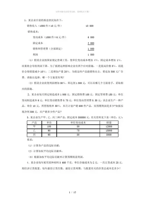
1、某企业目前的损益状况如在下:销售收入(1000件×10元/件) 10 000销售成本:变动成本(1000件×6元/件) 6 000固定成本 2 000销售和管理费(全部固定) 1 000利润 1 000(1)假设企业按国家规定普调工资,使单位变动成本增加4%,固定成本增加1%,结果将会导致利润下降。
为了抵销这种影响企业有两个应对措施:一是提高价格5%,而提价会使销量减少10%;二是增加产量20%,为使这些产品能销售出去,要追加500元广告费。
请做出选择,哪一个方案更有利?(2)假设企业欲使利润增加50%,即达到1 500元,可以从哪几个方面着手,采取相应的措施。
2、某企业每月固定制造成本1 000元,固定销售费100元,固定管理费150元;单位变动制造成本6元,单位变动销售费0.70元,单位变动管理费0.30元;该企业生产一种产品,单价10元,所得税税率50%;本月计划产销600件产品,问预期利润是多少?如拟实现净利500元,应产销多少件产品?3、某企业生产甲、乙、丙三种产品,固定成本500000元,有关资料见下表(单位:元):要求:(1)计算各产品的边际贡献;(2)计算加权平均边际贡献率;(3)根据加权平均边际贡献率计算预期税前利润。
4、某企业每年耗用某种材料3 600千克,单位存储成本为2元,一次订货成本25元。
则经济订货批量、每年最佳订货次数、最佳订货周期、与批量有关的存货总成本是多少?5.有10个同类企业的生产性固定资产年平均价值和工业总产值资料如下:(1)说明两变量之间的相关方向;(2)建立直线回归方程;(3)估计生产性固定资产(自变量)为1100万元时总产值(因变量)的可能值。
6、某商店的成本费用本期发生额如表所示,采用账户分析法进行成本估计。
首先,对每个项目进行研究,根据固定成本和变动成本的定义及特点结合企业具体情况来判断,确定它们属于哪一类成本。
例如,商品成本和利息与商店业务量关系密切,基本上属于变动成本;福利费、租金、保险、修理费、水电费、折旧等基本上与业务量无关,视为固定成本。
CHAPTER 7NETWORK OPTIMIZATION PROBLEMS Review Questions7.1-1 A supply node is a node where the net amount of flow generated is a fixed positive number.A demand node is a node where the net amount of flow generated is a fixed negativenumber. A transshipment node is a node where the net amount of flow generated is fixed at zero.7.1-2 The maximum amount of flow allowed through an arc is referred to as the capacity of thatarc.7.1-3 The objective is to minimize the total cost of sending the available supply through thenetwork to satisfy the given demand.7.1-4 The feasible solutions property is necessary. It states that a minimum cost flow problemwill have a feasible solution if and only if the sum of the supplies from its supply nodesequals the sum of the demands at its demand nodes.7.1-5 As long as all its supplies and demands have integer values, any minimum cost flowproblem with feasible solutions is guaranteed to have an optimal solution with integervalues for all its flow quantities.7.1-6 Network simplex method.7.1-7 Applications of minimum cost flow problems include operation of a distribution network,solid waste management, operation of a supply network, coordinating product mixes atplants, and cash flow management.7.1-8 Transportation problems, assignment problems, transshipment problems, maximum flowproblems, and shortest path problems are special types of minimum cost flow problems. 7.2-1 One of the company’s most important distribution centers (Los Angeles) urgently needs anincreased flow of shipments from the company.7.2-2 Auto replacement parts are flowing through the network from the company’s main factoryin Europe to its distribution center in LA.7.2-3 The objective is to maximize the flow of replacement parts from the factory to the LAdistribution center.7.3-1 Rather than minimizing the cost of the flow, the objective is to find a flow plan thatmaximizes the amount flowing through the network from the source to the sink.7.3-2 The source is the node at which all flow through the network originates. The sink is thenode at which all flow through the network terminates. At the source, all arcs point awayfrom the node. At the sink, all arcs point into the node.7.3-3 The amount is measured by either the amount leaving the source or the amount entering thesink.7.3-4 1. Whereas supply nodes have fixed supplies and demand nodes have fixed demands, thesource and sink do not.2. Whereas the number of supply nodes and the number of demand nodes in a minimumcost flow problem may be more than one, there can be only one source and only onesink in a standard maximum flow problem.7.3-5 Applications of maximum flow problems include maximizing the flow through adistribution network, maximizing the flow through a supply network, maximizing the flow of oil through a system of pipelines, maximizing the flow of water through a system ofaqueducts, and maximizing the flow of vehicles through a transportation network.7.4-1 The origin is the fire station and the destination is the farm community.7.4-2 Flow can go in either direction between the nodes connected by links as opposed to onlyone direction with an arc.7.4-3 The origin now is the one supply node, with a supply of one. The destination now is theone demand node, with a demand of one.7.4-4 The length of a link can measure distance, cost, or time.7.4-5 Sarah wants to minimize her total cost of purchasing, operating, and maintaining the carsover her four years of college.7.4-6 When “real travel” through a network can end at more that one node, a dummy destinationneeds to be added so that the network will have just a single destination.7.4-7 Quick’s management must consider trade-offs between time and cost in making its finaldecision.7.5-1 The nodes are given, but the links need to be designed.7.5-2 A state-of-the-art fiber-optic network is being designed.7.5-3 A tree is a network that does not have any paths that begin and end at the same nodewithout backtracking. A spanning tree is a tree that provides a path between every pair of nodes. A minimum spanning tree is the spanning tree that minimizes total cost.7.5-4 The number of links in a spanning tree always is one less than the number of nodes.Furthermore, each node is directly connected by a single link to at least one other node. 7.5-5 To design a network so that there is a path between every pair of nodes at the minimumpossible cost.7.5-6 No, it is not a special type of a minimum cost flow problem.7.5-7 A greedy algorithm will solve a minimum spanning tree problem.17.5-8 Applications of minimum spanning tree problems include design of telecommunicationnetworks, design of a lightly used transportation network, design of a network of high- voltage power lines, design of a network of wiring on electrical equipment, and design of a network of pipelines.Problems7.1a)b)c)1[40] 6 S17 4[-30] D1 [-40] D2 [60] 5 8S2 6[-30] D37.2a)supply nodestransshipment nodesdemand nodesb)[200] P1560 [150]425 [125][0] W1505[150]490 [100]470 [100][-150]RO1[-200]RO2P2 [300]c)510 [175]600 [200][0] W2390 [125]410[150] 440[75]RO3[-150]7.3a)supply nodestransshipment nodesdemand nodesV1W1F1V2V3W2 F21P1W1RO1RO2P2W2RO3[-50] SE3000[20][0]BN5700[40][0]HA[50]BE 4000 6300[40][30] [0][0]NY2000[60]2400[20]3400[10] 4200[80][0]5900[60]5400[40]6800[50]RO[0]BO[0]2500[70]2900[50]b)c)7.4a)LA 3100 NO 6100 LI 3200 ST[-130] [70] [30] [40] [130]1[70]11b)c) The total shipping cost is $2,187,000.7.5a)[0][0] 5900RONY[60] 5400[0] 2900 [50]4200 [80][0] [40] 6800 [50]BO[0] 2500LA 3100 NO 6100 LI 3200 ST [-130][70][30] [40][130]b)c)SEBNHABERONYNY(80) [80] (50) [60](30)[40] ROBO (40)(50) [50] (70)[70]11d)e)f) $1,618,000 + $583,000 = $2,201,000 which is higher than the total in Problem 7.5 ($2,187,000). 7.6LA(70) NO[50](30)LI (30) ST[70][30] [40]There are only two arcs into LA, with a combined capacity of 150 (80 + 70). Because ofthis bottleneck, it is not possible to ship any more than 150 from ST to LA. Since 150 actually are being shipped in this solution, it must be optimal. 7.7[-50] SE3000 [20] [0] BN 5700 [40][0] HA[50] BE4000 6300[40][0] NY2000 [60] 2400 [20][30] [0]5900RO [60]17.8 a) SourcesTransshipment Nodes Sinkb)7.9 a)AKR1[75]A [60]R2[65] [40][50][60] [45]D [120] [70]B[55]E[190]T [45][80] [70][70]R3CF[130][90]SE PT KC SL ATCHTXNOMES S F F CAb)Oil Fields Refineries Distribution CentersTXNOPTCACHATAKSEKCME c)SLSFTX[11][7] NO[5][9] PT[8] [2][5] CA [4] [7] [8] [7] [4] [6][8] CH [7][5][9] [4] ATAK [3][6][6][12] SE KC[8][9][4][8] [7] [12] [11]MESL [9]SF[15][7]d)3Shortest path: Fire Station – C – E – F – Farming Community 7.11 a)A70D40 60O60 5010 B 20 C5540 10 T50E801c)Shortest route: Origin – A – B – D – Destinationd)Yese)Yes7.12a)31,00018,000 21,00001238,000 10,000 12,000b)17.13a) Times play the role of distances.B 2 2 G5ACE 1 31 1b)7.14D F1. C---D: Cost = 14.E---G: Cost = 5E---F: Cost = 1 *choose arbitrarilyD---A: Cost = 4 2.E---G: Cost = 5 E---B: Cost = 7 E---B: Cost = 7 F---G: Cost = 7 E---C: Cost = 4 C---A: Cost = 5F---G: Cost = 7C---B: Cost = 2 *lowestF---C: Cost = 3 *lowest5.E---G: Cost = 5 F---D: Cost = 4 D---A: Cost = 43. E---G: Cost = 5 B---A: Cost = 2 *lowestE---B: Cost = 7 F---G: Cost = 7 F---G: Cost = 7 C---A: Cost = 5F---D: Cost = 46.E---G: Cost = 5 *lowestC---D: Cost = 1 *lowestF---G: Cost = 7C---A: Cost = 5C---B: Cost = 2Total = $14 million7.151. B---C: Cost = 1 *lowest 4. B---E: Cost = 72. B---A: Cost = 4 C---F: Cost = 4 *lowestB---E: Cost = 7 C---E: Cost = 5C---A: Cost = 6 D---F: Cost = 5C---D: Cost = 2 *lowest 5. B---E: Cost = 7C---F: Cost = 4 C---E: Cost = 5C---E: Cost = 5 F---E: Cost = 1 *lowest3. B---A: Cost = 4 *lowest F---G: Cost = 8B---E: Cost = 7 6. E---G: Cost = 6 *lowestC---A: Cost = 6 F---G: Cost = 8C---F: Cost = 4C---E: Cost = 5D---A: Cost = 5 Total = $18,000D---F: Cost = 57.16B 34 2E HA D 2 G I K3C F 12J34B41E6A C41G2 FD1. F---G: Cost = 1 *lowest 6. D---A: Cost = 62. F---C: Cost = 6 D---B: Cost = 5F---D: Cost = 5 D---C: Cost = 4F---I: Cost = 2 *lowest E---B: Cost = 3 *lowestF---J: Cost = 5 F---C: Cost = 6G---D: Cost = 2 F---J: Cost = 5G---E: Cost = 2 H---K: Cost = 7G---H: Cost = 2 I---K: Cost = 8G---I: Cost = 5 I---J: Cost = 33. F---C: Cost = 6 7. B---A: Cost = 4F---D: Cost = 5 D---A: Cost = 6F---J: Cost = 5 D---C: Cost = 4G---D: Cost = 2 *lowest F---C: Cost = 6G---E: Cost = 2 F---J: Cost = 5G---H: Cost = 2 H---K: Cost = 7I---H: Cost = 2 I---K: Cost = 8I---K: Cost = 8 I---J: Cost = 3 *lowestI---J: Cost = 3 8. B---A: Cost = 4 *lowest4. D---A: Cost = 6 D---A: Cost = 6D---B: Cost = 5 D---C: Cost = 4D---E: Cost = 2 *lowest F---C: Cost = 6D---C: Cost = 4 H---K: Cost = 7F---C: Cost = 6 I---K: Cost = 8F---J: Cost = 5 J---K: Cost = 4G---E: Cost = 2 9. A---C: Cost = 3 *lowestG---H: Cost = 2 D---C: Cost = 4I---H: Cost = 2 F---C: Cost = 6I---K: Cost = 8 H---K: Cost = 7I---J: Cost = 3 I---K: Cost = 85. D---A: Cost = 6 J---K: Cost = 4D---B: Cost = 5 10. H---K: Cost = 7D---C: Cost = 4 I---K: Cost = 8E---B: Cost = 3 J---K: Cost = 4 *lowestE---H: Cost = 4F---C: Cost = 6F---J: Cost = 5G---H: Cost = 2 *lowest Total = $26 millionI---H: Cost = 2I---K: Cost = 8I---J: Cost = 37.17a) The company wants a path between each pair of nodes (groves) that minimizes cost(length of road).b)7---8 : Distance = 0.57---6 : Distance = 0.66---5 : Distance = 0.95---1 : Distance = 0.75---4 : Distance = 0.78---3 : Distance = 1.03---2 : Distance = 0.9Total = 5.3 miles7.18a) The bank wants a path between each pair of nodes (offices) that minimizes cost(distance).b) B1---B5 : Distance = 50B5---B3 : Distance = 80B1---B2 : Distance = 100B2---M : Distance = 70B2---B4 : Distance = 120Total = 420 milesHamburgBostonRotterdamSt. PetersburgNapoliMoscowA IRFIELD SLondonJacksonvilleBerlin RostovIstanbulCases7.1a) The network showing the different routes troops and supplies may follow to reach the Russian Federation appears below.PORTSb)The President is only concerned about how to most quickly move troops and suppliesfrom the United States to the three strategic Russian cities. Obviously, the best way to achieve this goal is to find the fastest connection between the US and the three cities.We therefore need to find the shortest path between the US cities and each of the three Russian cities.The President only cares about the time it takes to get the troops and supplies to Russia.It does not matter how great a distance the troops and supplies cover. Therefore we define the arc length between two nodes in the network to be the time it takes to travel between the respective cities. For example, the distance between Boston and London equals 6,200 km. The mode of transportation between the cities is a Starlifter traveling at a speed of 400 miles per hour * 1.609 km per mile = 643.6 km per hour. The time is takes to bring troops and supplies from Boston to London equals 6,200 km / 643.6 km per hour = 9.6333 hours. Using this approach we can compute the time of travel along all arcs in the network.By simple inspection and common sense it is apparent that the fastest transportation involves using only airplanes. We therefore can restrict ourselves to only those arcs in the network where the mode of transportation is air travel. We can omit the three port cities and all arcs entering and leaving these nodes.The following six spreadsheets find the shortest path between each US city (Boston and Jacksonville) and each Russian city (St. Petersburg, Moscow, and Rostov).The spreadsheets contain the following formulas:Comparing all six solutions we see that the shortest path from the US to Saint Petersburg is Boston → London → Saint Petersburg with a total travel time of 12.71 hours. The shortest path from the US to Moscow is Boston → London → Moscow with a total travel time of 13.21 hours. The shortest path from the US to Rostov is Boston →Berlin → Rostov with a total travel time of 13.95 hours. The following network diagram highlights these shortest paths.-1c)The President must satisfy each Russian city’s military requirements at minimum cost.Therefore, this problem can be solved as a minimum-cost network flow problem. The two nodes representing US cities are supply nodes with a supply of 500 each (wemeasure all weights in 1000 tons). The three nodes representing Saint Petersburg, Moscow, and Rostov are demand nodes with demands of –320, -440, and –240,respectively. All nodes representing European airfields and ports are transshipment nodes. We measure the flow along the arcs in 1000 tons. For some arcs, capacityconstraints are given. All arcs from the European ports into Saint Petersburg have zero capacity. All truck routes from the European ports into Rostov have a transportation limit of 2,500*16 = 40,000 tons. Since we measure the arc flows in 1000 tons, the corresponding arc capacities equal 40. An analogous computation yields arc capacities of 30 for both the arcs connecting the nodes London and Berlin to Rostov. For all other nodes we determine natural arc capacities based on the supplies and demands at the nodes. We define the unit costs along the arcs in the network in $1000 per 1000 tons (or, equivalently, $/ton). For example, the cost of transporting 1 ton of material from Boston to Hamburg equals $30,000 / 240 = $125, so the costs of transporting 1000 tons from Boston to Hamburg equals $125,000.The objective is to satisfy all demands in the network at minimum cost. The following spreadsheet shows the entire linear programming model.HamburgBoston Rotterdam St.Petersburg+500-320Napoli Moscow A IRF IELDSLondon -440Jacksonville Berlin Rostov+500-240Istanbul The total cost of the operation equals $412.867 million. The entire supply for SaintPetersburg is supplied from Jacksonville via London. The entire supply for Moscow is supplied from Boston via Hamburg. Of the 240 (= 240,000 tons) demanded by Rostov, 60 are shipped from Boston via Istanbul, 150 are shipped from Jacksonville viaIstanbul, and 30 are shipped from Jacksonville via London. The paths used to shipsupplies to Saint Petersburg, Moscow, and Rostov are highlighted on the followingnetwork diagram.PORTSd)Now the President wants to maximize the amount of cargo transported from the US tothe Russian cities. In other words, the President wants to maximize the flow from the two US cities to the three Russian cities. All the nodes representing the European ports and airfields are once again transshipment nodes. The flow along an arc is againmeasured in thousands of tons. The new restrictions can be transformed into arccapacities using the same approach that was used in part (c). The objective is now to maximize the combined flow into the three Russian cities.The linear programming spreadsheet model describing the maximum flow problem appears as follows.The spreadsheet shows all the amounts that are shipped between the various cities. The total supply for Saint Petersburg, Moscow, and Rostov equals 225,000 tons, 104,800 tons, and 192,400 tons, respectively. The following network diagram highlights the paths used to ship supplies between the US and the Russian Federation.PORTSHamburgBoston Rotterdam St.Petersburg+282.2 -225NapoliMoscowAIRFIELDS-104.8LondonJacksonvilleBerlin Rostov +240 -192.4Istanbule)The creation of the new communications network is a minimum spanning tree problem.As usual, a greedy algorithm solves this type of problem.Arcs are added to the network in the following order (one of several optimal solutions):Rostov - Orenburg 120Ufa - Orenburg 75Saratov - Orenburg 95Saratov - Samara 100Samara - Kazan 95Ufa – Yekaterinburg 125Perm – Yekaterinburg 857.2a) There are three supply nodes – the Yen node, the Rupiah node, and the Ringgit node.There is one demand node – the US$ node. Below, we draw the network originatingfrom only the Yen supply node to illustrate the overall design of the network. In thisnetwork, we exclude both the Rupiah and Ringgit nodes for simplicity.b)Since all transaction limits are given in the equivalent of $1000 we define the flowvariables as the amount in thousands of dollars that Jake converts from one currencyinto another one. His total holdings in Yen, Rupiah, and Ringgit are equivalent to $9.6million, $1.68 million, and $5.6 million, respectively (as calculated in cells I16:K18 inthe spreadsheet). So, the supplies at the supply nodes Yen, Rupiah, and Ringgit are -$9.6 million, -$1.68 million, and -$5.6 million, respectively. The demand at the onlydemand node US$ equals $16.88 million (the sum of the outflows from the sourcenodes). The transaction limits are capacity constraints for all arcs leaving from thenodes Yen, Rupiah, and Ringgit. The unit cost for every arc is given by the transactioncost for the currency conversion.Jake should convert the equivalent of $2 million from Yen to each US$, Can$, Euro, and Pound. He should convert $1.6 million from Yen to Peso. Moreover, he should convert the equivalent of $200,000 from Rupiah to each US$, Can$, and Peso, $1 million from Rupiah to Euro, and $80,000 from Rupiah to Pound. Furthermore, Jake should convert the equivalent of $1.1 million from Ringgit to US$, $2.5 million from Ringgit to Euro, and $1 million from Ringgit to each Pound and Peso. Finally, he should convert all the money he converted into Can$, Euro, Pound, and Peso directly into US$. Specifically, he needs to convert into US$ the equivalent of $2.2 million, $5.5 million, $3.08 million, and $2.8 million Can$, Euro, Pound, and Peso, respectively. Assuming Jake pays for the total transaction costs of $83,380 directly from his American bank accounts he will have $16,880,000 dollars to invest in the US.c)We eliminate all capacity restrictions on the arcs.Jake should convert the entire holdings in Japan from Yen into Pounds and then into US$, the entire holdings in Indonesia from Rupiah into Can$ and then into US$, and the entire holdings in Malaysia from Ringgit into Euro and then into US$. Without the capacity limits the transaction costs are reduced to $67,480.d)We multiply all unit cost for Rupiah by 6.The optimal routing for the money doesn't change, but the total transaction costs are now increased to $92,680.e)In the described crisis situation the currency exchange rates might change every minute.Jake should carefully check the exchange rates again when he performs thetransactions.The European economies might be more insulated from the Asian financial collapse than the US economy. To impress his boss Jake might want to explore other investment opportunities in safer European economies that provide higher rates of return than US bonds.。
《数据模型与决策》复习题及参考答案《数据模型与决策》复习题及参考答案第一章绪言一、填空题1.运筹学的主要研究对象是各种有组织系统的管理问题,经营活动。
2.运筹学的核心是运用数学方法研究各种系统的优化途径及方案,为决策者提供科学决策的依据。
3.模型是一件实际事物或现实情况的代表或抽象。
4、通常对问题中变量值的限制称为约束条件,它可以表示成一个等式或不等式的集合。
5.运筹学研究和解决问题的基础是最优化技术,并强调系统整体优化功能。
运筹学研究和解决问题的效果具有连续性。
6.运筹学用系统的观点研究功能之间的关系。
7.运筹学研究和解决问题的优势是应用各学科交叉的方法,具有典型综合应用特性。
8.运筹学的发展趋势是进一步依赖于_计算机的应用和发展。
9.运筹学解决问题时首先要观察待决策问题所处的环境。
10.用运筹学分析与解决问题,是一个科学决策的过程。
11.运筹学的主要目的在于求得一个合理运用人力、物力和财力的最佳方案。
12.运筹学中所使用的模型是数学模型。
用运筹学解决问题的核心是建立数学模型,并对模型求解。
13用运筹学解决问题时,要分析,定议待决策的问题。
14.运筹学的系统特征之一是用系统的观点研究功能关系。
15.数学模型中,“s〃t”表示约束。
16.建立数学模型时,需要回答的问题有性能的客观量度,可控制因素,不可控因素。
17.运筹学的主要研究对象是各种有组织系统的管理问题及经营活动。
二、单选题1.建立数学模型时,考虑可以决策者控制的因素是第 1 页共40页A.销售数量B.销售价格C.顾客的需求D.竞争价格 2.我们可以通过来验证模型最优解。
A.观察B.应用C.实验D.调查 3.建立运筹学模型的过程不包括阶段。
A.观察环境B.数据分析C.模型设计D.模型实施 4.建立模型的一个基本理是去揭晓那些重要的或有关的 A数量B变量 C 约束条件 D 目标函数5.模型中要求变量取值A可正B可负C非正D非负 6.运筹学研究和解决问题的效果具有A 连续性B 整体性C 阶段性D 再生性7.运筹学运用数学方法分析与解决问题,以达到系统的最优目标。
数据模型与决策期末考试试卷(合肥工业大学)----c299fdee-6eb3-11ec-b318-7cb59b590d7d合肥工业大学工商管理硕士(mba)试卷(试卷a)课程名称:数据模型和决策命题教师:杨爱峰测试类别:开卷考试类:13MBA Spring Tunes 2类考试日期:2022年7月27日试题:一、(10分)库兹公司制造产品1和产品2,两种产品需经过两个部门的制造过程。
下表是两种产品的利润贡献及消耗人工工时的数据。
下一个生产周期内,公司总共有900小时的可用人工工时分配到两个部门。
试建立一个生产计划,使其目标为目标1(第一优先级目标):利润至少10000美元;目标2(第二优先目标):两个部门使用的工时应尽可能相等。
注:仅建立模型,未解决产品12二、(10分)合肥艺术馆打算安装一个摄像安全系统以减少其保安费用。
合肥艺术馆共有8间展厅(房间1-房间8),展厅之间的通道为1-13(见下图)。
一家摄像安装公司建议在一些通道处安装双向摄像头,以起到监测通道两侧房间的作用。
例如,在通道4安装,可以监测房间1和房间4。
管理层不打算在艺术馆入口处安装摄像头,并且认为房间7中展览的物品很重要,房间7至少有两个摄像头覆盖。
问应该如何安装最小数目的摄像头使其能够监测到每个房间?注:只建模型,不用求解单位利润(美元)250200工时(小时)a部门611b部门1210三、(10分)安绿电子是一家电子公司,有两家生产工厂,分别记为工厂1和工厂2,从每个工厂生产出来的产品都被运到公司的中转仓库1或者中转仓库2中,再通过中转仓库将其一产品运往三个零售商处。
工厂的供给量,零售商的需求量,以及工厂和中转仓库、中转仓库和零售商之间的单位运输成本见下表。
问如何安排运输方案使得工厂到零售商的运费最省?注:只建模型,不用求解工厂运输成本工厂1工厂2中转仓库运输成本中转仓库1中转仓库2需求量四、(10分)迈宇公司正在考虑如何管理其数据处理操作系统。

数据模型与决策试卷一、建模计算分析题(30分)下面两个题目任选一个做即可1艾伦是一个个人投资者,有70000美元可用于不同的投资。
不同投资的年回报率分别为:政府债券8.5%,存款5%,短期国库券6.5%,增长股基金13%。
所有的投资都要满1年后才对收益进行评估。
然而,每项投资都会有不同的风险,因此建议进行多元投资。
艾伦想知道每项投资各位多少可以使收益最大化。
下面的方针可以使投资具有多样性,从而降低投资者的风险:(1)对政府债券的投资比例不要超过全部投资的20%。
(2)在存款方面的投资不要超过其他3种投资的总和。
(3)在存款和短期国库券方面的投资至少要占全部投资的30%(4)为了投资安全,在存款和短期国库券方面的投资与在政府债券和增长股基金方面的投资比例至少是1.2:1。
(5)艾伦想把70000美元全部用来投资。
如果全部投资不再正好是70000美元,其他条件不变,则模型应该如何变化?2某投资咨询公司,为大量的客户管理高达1.2亿元的资金。
公司运用一个很有价值的模型,为每个客户安排投资量,分别投资在股票增长基金、收入基金和货币市场基金。
为了保证客户投资的多元化,公司对这三种投资的数额加以限制。
一般来说,投资在股票方面的资金应该占总投资的20%~40%,投资在收入基金方面的资金应该确保在20%~50%,货币市场方面的投资至少应该占30%。
此外,公司还尝试着引入了风险承受能力指数,以迎合不同投资者的需求。
如该公司的一位新客户希望投资800000元。
对其风险承受能力进行评估得出其风险指数为0.05。
公司的风险分析人员计算出,股票市场的风险指数是0.10,收入基金的风险指数是0.07,货币市场的风险指数是0.01,整个投资的风险指数是各项投资占投资的百分率与其风险指数乘积的代数和。
此外该公司预测股票基金的年收益是18%,收入基金的收益率是12.5%,货币市场基金的收益率是7.5%。
现在基于以上信息,公司应该如何安排这位客户的投资呢?建立线性规划模型,求出使总收益最大的解,并根据模型写出管理报告。
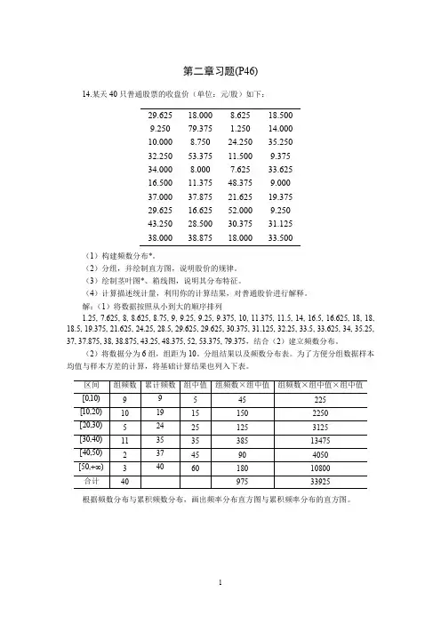
第二章习题(P46)14.某天40只普通股票的收盘价(单位:元/股)如下:29.625 18.000 8.625 18.5009.250 79.375 1.250 14.00010.000 8.750 24.250 35.25032.250 53.375 11.500 9.37534.000 8.000 7.625 33.62516.500 11.375 48.375 9.00037.000 37.875 21.625 19.37529.625 16.625 52.000 9.25043.250 28.500 30.375 31.12538.000 38.875 18.000 33.500(1)构建频数分布*。
(2)分组,并绘制直方图,说明股价的规律。
(3)绘制茎叶图*、箱线图,说明其分布特征。
(4)计算描述统计量,利用你的计算结果,对普通股价进行解释。
解:(1)将数据按照从小到大的顺序排列1.25, 7.625, 8, 8.625, 8.75, 9, 9.25, 9.25, 9.375, 10, 11.375, 11.5, 14, 16.5, 16.625, 18, 18, 18.5, 19.375, 21.625, 24.25, 28.5, 29.625, 29.625, 30.375, 31.125, 32.25, 33.5, 33.625, 34, 35.25, 37, 37.875, 38, 38.875, 43.25, 48.375, 52, 53.375, 79.375,结合(2)建立频数分布。
(2)将数据分为6组,组距为10。
分组结果以及频数分布表。
为了方便分组数据样本均值与样本方差的计算,将基础计算结果也列入下表。
根据频数分布与累积频数分布,画出频率分布直方图与累积频率分布的直方图。
频率分布直方图从频率直方图和累计频率直方图可以看出股价的规律。
股价分布10元以下、10—20元、30—40元占到60%,股价在40元以下占87.5%,分布不服从正态分布等等。
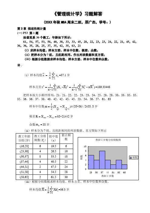
《管理统计学》习题解答(20XX 年秋MBA 周末二班,邢广杰,学号:)第3章 描述性统计量 (一) P53 第1题抽查某系30个教工,年龄如下所示:61,54,57,53,56,40,38,33,33,45,28,22,23,23,24,22,21,45,42,36,36,35,28,25,37,35,42,35,63,21(i )求样本均值、样本方差、样本中位数、极差、众数;(ii )把样本分为7组,且组距相同。
作出列表数据和直方图; (iii )根据分组数据求样本均值、样本方差、样本中位数和众数。
解:(i )样本均值∑==n1i ixn1x =37.1岁样本方差)X n X (1-n 1)X (X 1-n 1s 2n 1i 2i2n 1i i 2-=-=∑∑===189.33448 把样本按大小顺序排列:21,21,22,22,23,23,24,25,28,28,33,33,35,35,35,36,36,37,38,40,42,42,45,45,53,54,56,57,61,63样本中位数)X X (21m 1)2n ()2n (++==(35+36)/2=35.5岁极差=-=1)()n (X X R 63-21=42岁 众数=0m 35岁(ii )样本分为7组、且组距相同的列表数据、直方图如下所示样本均值i k1i f Xi n 1X ∑===36.3岁样本方差)X n f X (1-n 1f )X (X 1-n 1s 2k 1i i 2i i2k 1i i 2-=-=∑∑===174.3724 样本中位数810230730f F 2n i I m -+=-+==34.375岁 众数=--⨯-+=---+=+448248730f f 2f f f iI m 1m 1-m m 1-m m 033.5岁(二)P53 第2题某单位统计了不同级别的员工的月工资水平资料如下:解:样本均值i k1i f Xi n 1X ∑===1566.667元样本标准差)X n f X (1-n 1f )X (X 1-n 1s 2k 1i i2i i 2k 1i i -=-=∑∑===398.1751元 样本中位数在累计74人的那一组,m=1500元; 众数1500m 0=元。
MBA数据模型与决策考卷一、选择题(每题2分,共20分)A. 变量B. 参数C. 数据源D. 数据分析工具A. 信息增益B. 权重C. 相关性D. 方差A. 线性回归模型B. 逻辑回归模型C. 神经网络模型D. 决策树模型A. 目标函数B. 约束条件C. 变量非负D. 变量连续A. 加权评分模型B. 层次分析法C. 数据包络分析法D. 主成分分析法A. 欧氏距离B. 曼哈顿距离C. 杰卡德距离D. 马氏距离A. 移动平均法B. 指数平滑法C. 自回归移动平均模型D. 聚类分析法A. 敏感度B. 确定性C. 稳定性D. 风险A. 数据库B. 模型库C. 知识库D. 网络库A. 净现值B. 内部收益率C. 投资回收期D. 利润率二、简答题(每题10分,共30分)1. 简述数据模型的分类及其特点。
2. 请阐述决策树的基本原理及其在商业决策中的应用。
3. 简述线性规划与非线性规划的区别。
三、计算题(每题15分,共30分)1. 某企业生产两种产品,产品A的利润为10元/件,产品B的利润为15元/件。
生产一件产品A需要2小时,生产一件产品B需要3小时。
企业每月共有240小时的生产时间,且市场需求量分别为100件和80件。
请用线性规划方法求解该企业如何分配生产时间以获得最大利润。
数据:{1, 2, 3, 4, 5, 6, 7, 8, 9, 10}四、案例分析题(20分)某电商企业想要提高用户转化率,现有一份用户行为数据,包括用户年龄、性别、浏览时长、次数、购买次数等。
请结合数据模型与决策方法,为该企业提出一套提高用户转化率的策略。
五、论述题(10分)请结合实际案例,论述数据模型与决策在企业战略管理中的应用价值。
一、选择题答案1. D2. A3. C4. D5. D6. A7. D8. A9. D10. A二、简答题答案1. 数据模型分类及特点:统计模型:基于概率论和统计学原理,特点是可以处理不确定性数据。
优化模型:基于数学规划,特点是可以求解最优解。
数据、模型与决策习题一、判断题(你认为下列命题是否正确, 对正确的打“√”;错误的打“×”) 1..若线性规划无最优解则其可行域无界.. ) 2.在邻接矩阵中, 全零的列所对应的点为汇点..) 3.线性规划的最优解一定是基本最优解.. )4.可行解集非空时, 则在极点上(凸多边形顶点)至少有一点达到最优....)5.基本解对应的基是可行... )6. 线性规划的最优解是基本解( )7. 可行解是基本解( )8.单纯形法计算中, 选取检验数为最大正数对应的 作为进基变量, 将使目标函数值得到最快的增长.. )9.在给定显著性水.. 下,,........ 时,拒绝即可认为 与 之间确有线性关系( ) 10.凡基本解一定是可行解.. ) 11.正反馈系统具有自我增强功能...)12.选取检验数为最小值对应的 作为进基变量, 将使目标函数值得到最快的增长...) 13.马尔柯夫链的特性为: 事物的第n 次实验结果仅取决于(n-1)次实验结果...) 14.对于非确定性问题, 无论采取何种预测方法, 也不可能得到精确的预测结果...) 15.可达矩阵表明了各点长度不大于n-1通路的可达情况.. )16.在采用层次分析法评价过程中, 由专家构造的判断矩阵也必须进行一致性检验...) 17.决策的定义是:从若干个备选方案中选择一个最优的(满意)方案, 并加以实施.. ) 18.科学决策就是依靠决策者的个人阅历、知识和智慧来对可行方案进行选择的过程. ) 19.小中取大原则—悲观原则, 是一种悲观保守的决策策略, 而大中取大原则—乐观原则才是一种积极进取的决策策....................... . )20.决策树针对的是具有风险性特征事物的一种决策方法. ) 二、填空题1 一元线性回归模型是( ), 其中 ( )是自变量, ( )是因变量, ( 和 )是( )。
y ˆk x x x ,,,212 由 , 得出 , , 其中 等于( ), 等于( ), 则用于一元线性回归模型 , 表示为( )。
教材习题答案1.2 工厂每月生产A 、B 、C 三种产品 ,单件产品的原材料消耗量、设备台时的消耗量、资源限量及单件产品利润如表1-22所示.和130.试建立该问题的数学模型,使每月利润最大.【解】设x 1、x 2、x 3分别为产品A 、B 、C 的产量,则数学模型为123123123123123max 1014121.5 1.2425003 1.6 1.21400150250260310120130,,0Z x x x x x x x x x x x x x x x =++++≤⎧⎪++≤⎪⎪≤≤⎪⎨≤≤⎪⎪≤≤⎪≥⎪⎩ 1.3 建筑公司需要用6m 长的塑钢材料制作A 、B 两种型号的窗架.两种窗架所需材料规格及数量如表1-23所示:【解】 设x j (j =1,2,…,14)为第j 种方案使用原材料的根数,则 (1)用料最少数学模型为14112342567891036891112132347910121314min 2300322450232400232346000,1,2,,14jj j Z x x x x x x x x x x x x x x x x x x x x x x x x x x x x x j ==⎧+++≥⎪++++++≥⎪⎪++++++≥⎨⎪++++++++≥⎪⎪≥=⎩∑ 用单纯形法求解得到两个基本最优解X (1)=( 50 ,200 ,0 ,0,84 ,0,0 ,0 ,0 ,0 ,0 ,200 ,0 ,0 );Z=534 X (2)=( 0 ,200 ,100 ,0,84 ,0,0 ,0 ,0 ,0 ,0 ,150 ,0 ,0 );Z=534 (2)余料最少数学模型为134131412342567891036891112132347910121314min 0.60.30.70.40.82300322450232400232346000,1,2,,14j Z x x x x x x x x x x x x x x x x x x x x x x x x x x x x x x x x x j =+++++⎧+++≥⎪++++++≥⎪⎪++++++≥⎨⎪++++++++≥⎪⎪≥=⎩ 用单纯形法求解得到两个基本最优解X (1)=( 0 ,300 ,0 ,0,50 ,0,0 ,0 ,0 ,0 ,0 ,200 ,0 ,0 );Z=0,用料550根 X (2)=( 0 ,450 ,0 ,0,0 ,0,0 ,0 ,0 ,0 ,0 ,200 ,0 ,0 );Z=0,用料650根 显然用料最少的方案最优。
数据模型与决策试卷一、建模计算分析题(30分)下面两个题目任选一个做即可1艾伦是一个个人投资者,有70000美元可用于不同的投资。
不同投资的年回报率分别为:政府债券8.5%,存款5%,短期国库券6.5%,增长股基金13%。
所有的投资都要满1年后才对收益进行评估。
然而,每项投资都会有不同的风险,因此建议进行多元投资。
艾伦想知道每项投资各位多少可以使收益最大化。
下面的方针可以使投资具有多样性,从而降低投资者的风险:(1)对政府债券的投资比例不要超过全部投资的20%。
(2)在存款方面的投资不要超过其他3种投资的总和。
(3)在存款和短期国库券方面的投资至少要占全部投资的30%(4)为了投资安全,在存款和短期国库券方面的投资与在政府债券和增长股基金方面的投资比例至少是1.2:1。
(5)艾伦想把70000美元全部用来投资。
如果全部投资不再正好是70000美元,其他条件不变,则模型应该如何变化?2某投资咨询公司,为大量的客户管理高达1.2亿元的资金。
公司运用一个很有价值的模型,为每个客户安排投资量,分别投资在股票增长基金、收入基金和货币市场基金。
为了保证客户投资的多元化,公司对这三种投资的数额加以限制。
一般来说,投资在股票方面的资金应该占总投资的20%~40%,投资在收入基金方面的资金应该确保在20%~50%,货币市场方面的投资至少应该占30%。
此外,公司还尝试着引入了风险承受能力指数,以迎合不同投资者的需求。
如该公司的一位新客户希望投资800000元。
对其风险承受能力进行评估得出其风险指数为0.05。
公司的风险分析人员计算出,股票市场的风险指数是0.10,收入基金的风险指数是0.07,货币市场的风险指数是0.01,整个投资的风险指数是各项投资占投资的百分率与其风险指数乘积的代数和。
此外该公司预测股票基金的年收益是18%,收入基金的收益率是12.5%,货币市场基金的收益率是7.5%。
现在基于以上信息,公司应该如何安排这位客户的投资呢?建立线性规划模型,求出使总收益最大的解,并根据模型写出管理报告。
《数据、模型与决策》案例案例1 北方化工厂月生产计划安排(0.7+0.3)一. 问题提出根据经营现状和目标,合理制定生产计划并有效组织生产,是一个企业提高效益的核心。
特别是对于一个化工厂而言,由于其原料品种多,生产工艺复杂,原材料和产成品存储费用较高,并有一定的危险性,对其生产计划作出合理安排就显得尤为重要。
现要求我们对北方化工厂的生产计划做出合理安排。
二. 有关数据1.生产概况北方化工厂现在有职工120人,其中生产工人105名。
主要设备是2套提取生产线,每套生产线容量为800kg,至少需要10人看管。
该工厂每天24小时连续生产,节假日不停机。
原料投入到成品出线平均需要10小时,成品率约为60%,该厂只有4吨卡车1辆,可供原材料运输。
2.产品结构及有关资料该厂目前的产品可分为5类,多有原料15种,根据厂方提供的资料,经整理得表1。
3.供销情况①根据现有运出条件,原料3从外地购入,每月只能购入1车。
②根据前几个月的销售情况,产品1和产品3应占总产量的70%,产品2的产量最好不要超过总产量的5%,产品1的产量不要低于产品3与产品4的产量之和。
问题:a.请作该厂的月生产计划,使得该厂的总利润最高。
b.找出阻碍该厂提高生产能力的瓶颈问题,提出解决办法。
案例2 石华建设监理公司监理工程师配置问题(0.8+0.2)石华建设监理公司(国家甲级),侧重国家大中型项目的监理,仅在河北省石家庄市就正在监理七项工程,总投资均在5000万元以上。
由于工程开工的时间不同,多工程工期之间相互搭接,具有较长的连续性,2012年监理的工程量与2011年监理的工程量大致相同。
每项工程安排多少监理工程师进驻工地,一般是根据工程的投资,建筑规模,使用功能,施工的形象进度,施工阶段来决定的。
监理工程师的配置数量是随之而变化的。
由于监理工程师从事的专业不同,他们每人承担的工作量也是不等的。
有的专业一个工地就需要三人以上,而有的专业一人则可以兼管三个以上的工地。
14-1 CHAPTER 14QUEUEING MODELSReview Questions14.1-1 Customers might be vehicles, machines, or other items.14.1-2 It might be a crew of people working together, a machine, a vehicle, or an electronicdevice. 14.1-3 Mean arrival rate = 1 / (mean interarrival time). 14.1-4Time14.1-5 The mean equals the standard deviation of the exponential distribution.14.1-6 Having random arrivals means that arrival times are completely unpredictable in thesense that the chance of an arrival in the next minute always is just the same as for any other minute. The only distribution of interarrival times that fits having random arrivals is the exponential distribution. 14.1-7 The number of customers in the queue is the number of customers waiting forservice to begin. The number of customers in the system is the number in the queue plus the number currently being served. 14.1-8 Queueing models conventionally assume that the queue is an infinite queue andthat the queue discipline is first come first served. 14.1-9 Mean service time = 1 / (mean service rate).14.1-10 For the exponential distribution, the standard deviation equals the mean. For thedegenerate distribution, the standard deviation equals zero. For the Erlangdistribution, the standard deviation =1k(mean).14.1-11 The three parts of a label for queueing models provide information on thedistribution of service times, the number of servers, and the distribution ofinterarrival times.14.2-1 In commercial service systems, outside customers receive service from commercialorganizations. Many examples are possible.14.2-2 In internal service systems, the customers receiving service are internal to theorganization. Many examples are possible.14.2-3 In transportation service systems, either the customers or the servers are vehicles.Many examples are possible.14.3-1 When the customers are internal to the organization providing the service, it ismore important how many customers typically are waiting in the queueing system.14.3-2 Commercial service systems tend to place a greater importance on how longcustomers typically have to wait.14.3-3 L= expected number of customers in the systemL q= expected number of customers in the queue W= expected waiting time in the system W q = expected waiting time in the queue14.3-4 A queueing system is in a steady state condition if it is in its normal condition afteroperating for some time.14.3-5 W = W q + (1/μ)14.3-6 L = λW and L q = λW q14.3-7 L = L q + (λ / μ)14.3-8 Steady-state probabilities can also be used as measures of performance.14.4-1 Each Tech Rep should be assigned enough machines so that the Tech Rep will beactive repairing machines approximately 75% of the time.14.4-2 The issue is the increased number of complaints about intolerable waits for repairson the new copier.14.4-3 The average waiting time of customers before the Tech Rep begins the trip to thecustomer site to repair the machine should not exceed two hours.14.4-4 Four alternative approaches have been suggested.14.4-5 A team of management scientist and John Phixitt will analyze these approaches. 14.4-6 The machines needing repair are the customers and the Tech Reps are the servers.14-214.5-1 λ= expected number of arrivals per unit timeμ= expected number of service completions per unit time (1/λ) = expected interarrival time (1/μ) = expected service time ρ = utilization factor14.5-2 (1) Interarrival times have an exponential distribution with a mean of (1/λ); (2) servicetimes have an exponential distribution with a mean of (1/μ); (3) the queueing system has 1 server.14.5-3 Formulas are available for L, W, W q, L q, P n, P(W>t), P(W q>t), and P(W q=0).14.5-4 ρ < 114.5-5 The average waiting time until service begins is 6 hours.14.5-6 It would cost approximately $300 million annually.14.5-7 The M/G/1 model differs in the assumption about service time. In this model theservice times can have any probability distribution. It is not even necessary to determine the form of this distribution. It is only necessary to estimate the mean and standard deviation of the distribution.14.5-8 The M/D/1 model assumes a degenerate service-time distribution. The M/E k/1model assumes an Erlang distribution with shape parameter k.14.5-9 Decreasing the standard deviation decreases L q, L, W, and W q.14.5-10 The total additional cost is a one-time cost of approximately $500 million.14.6-1 ρ = λ / (sμ) which is the average fraction of time that individual servers are beingutilized serving customers.14.6-2 ρ < 114.6-3 Explicit formulas are available for all the measures of performance considered forthe M/M/1 model.14.6-4 Three territories need to be combined in order to satisfy the new service standard.14.6-5 The M/M/s model has a great amount of variability in service times. The M/D/smodel has no variability. The M/E k/s model provides a middle ground between the other two with some variability in service times.14.7-1 When using priorities, more important customers are served ahead of others whohave waited longer.14-314.7-2 With nonpreemptive priorities, once a server has begun serving a customer, theservice must be completed without interruption even if a higher priority customer arrives while this service is in process. With preemptive priorities, the lowest priority customer being served is ejected back into the queue whenever a higher priority customer enters the queueing system.14.7-3 Except for using preemptive priorities, the assumptions are the same as for theM/M/1 model.14.7-4 Except for using nonpreemptive priorities, the assumptions are the same as for theM/M/s model.14.7-5 ρ < 114.7-6 Priority class 1 consists of printer-copiers and priority class 2 consists of all othermachines.14.7-7 Two-person territories would be needed to reduce waiting times to acceptablelevels.14.7-8 Management decided to change to two-person territories, with priority given to theprinter-copiers for repairs.14.8-1 Giving a relatively high utilization factor to the server provides surprisingly poormeasures of performance for the system.14.8-2 As ρ is increased above 0.9, L q and L grow astronomically.14.8-3 Decreasing the variability of service times improves the performance of a single-server queueing system substantially.14.8-4 Cutting the variability of service times in half provides most of the improvementfrom completely eliminating the variability.14.8-5 Combining separate single-server queueing systems into one multiple-serverqueueing system greatly improves the measures of performance.14.8-6 Applying priorities when selecting customers to begin service can greatly improvethe measures of performance for high-priority customers.14.8-7 Applying preemptive priorities improves the measures of performance forcustomers in the top priority class even more than applying nonpreemptive priorities.14.9-1 When choosing the number of servers there is a tradeoff between the cost of theservers and the amount of waiting by the customers.14-414.9-2 Making one’s own employees wait causes lost productivity, which results in lostprofit which is the waiting cost.14.9-3 Waiting Cost = C w L where C w is the waiting cost per unit time for each customer inthe queueing system, and L is the expected number of customers in the queueing system.14.9-4 A relatively high utilization factor for the servers in a queueing system can actuallybe more costly and therefore not advisable.14.10-1 Previous one-person territories were replaced by larger three-person territories.14.10-2 Queueing models were used to find the minimum number of servers that wouldprovide satisfactory measures of performance for the queueing system.14.10-3 Decisions needed to be made on the number of telephone trunk lines, telephoneagents, and hold positions.14.10-4 The city’s arrestees were the customers in New York City.14.10-5 More than $750 million in annual profits were obtained by the business customersof AT&T.14.10-6 A special kind of queueing system where the customers (the printers to beassembled) go through a series of servers (assembly operations) in a fixed sequence. Problems14.1 a) A hospital emergency room is a queueing system with patients as the customersand care providers as the servers.b) The queue is the waiting room and it would operate on a priority procedure.c) Arrivals would be random since arrival times are completely unpredictable.d) The service times in this context would be the amount of time it takes for a patientto receive care, which would be highly variable.14.214-514.3 a) True. The only distribution of interarrival times that fits having random arrivals isthe exponential distribution.b) False. The probability of an arrival in the next minute is completely uninfluencedby when the last arrival occurred.c) True. Most queueing models assume that the form of the probability distributionof interarrival times is an exponential distribution.14.4 a) False. Depending on the nature of the queueing system, the exponentialdistribution can provide either a reasonable approximation or a gross distortion ofthe true service-time distribution.b) False. The mean and standard deviation are always equal.c) True. The exponential and degenerate distributions represent two rather extremecases regarding the amount of variability in the service times.14.5 a) False. The queue is where customers wait before being served.b) False. Queueing models conventionally assume that the queue is an infinitequeue.c) True. The most common is first-come-first-served.14.6 a) A bank is a queueing system with people as the customers, and tellers as theservers.b) W q= 1 minuteW= W q+ (1/μ) = 1 + 2 = 3 minutesL q= λW q= (40/60 per minute) (1 minute) = 0.667 customersL = λW = (40/60 customers per minute) (3 minutes) = 2 customers14-614.7 a) A parking lot is a queueing system for providing parking with cars as thecustomers, and parking spaces as the servers. The service time is the amount oftime a car spends in a space. The queue capacity is 0.b) L= 0P0+ 1P1+ 2P2+ 3P3= 0(0.2) + 1(0.3) + 2(0.3) + 3(0.2) = 1.5 carsL q= 0 carsW= L / λ= 1.5 / 2 = 0.75 hoursW q = L q / λ = 0 / 2 = 0 hoursc) A car spends an average of 45 minutes in a parking space.14.8 a) L= 0(1/16) + 1(4/16) + 2(6/16) + 3(4/16) + 4(1/16) = 2, which represents theaverage number of customers in the shop, including those getting their hair cut.b)n # in queue probability product0 01 02 03 1 0.25 0.254 2 0.0625 0.125L q = 0.375 which represents the average number of customers in the shop waitingto get a haircut.c) W= L/λ= 2/4 = 0.5 hours = 30 minutesW q= L q/l= 0.375/4 = 0.094 hours = 5.625 minutesThese quantities mean that customers will be in the shop an average of half anhour, including the time to get a haircut, and will have to wait an average of 5.625minutes before their haircut will begin.d) W - W q = 0.5 – 0.094 = 0.406 hours = 24.375 minutes14.9 The utilization factor ρ represents the fraction of time that the server is busy. Theserver is busy except when there are zero people in the system. P0 is the probability of having 0 customers in the system. Hence, ρ = 1 –P0.14-714.10 a) L= λ/(μ–λ) = 30/(40–30) = 3 customersW= 1/(μ-λ)= 1/(40–30) = 0.1 hoursW q= λ/[μ(μ-λ)] = 30/[40(40–30)] = 0.075 hoursL q= λW q= 30(0.075) = 2.25 customersP0= 1–ρ= 1–0.75 = 0.25P1= (1–ρ)ρ= (1–0.75)(0.75) = 0.188P2= (1–ρ)ρ2= (1–0.75)(0.75)2= 0.141There is a 1–P0–P1–P2 = 1–0.25–0.188–0.141 = 42% chance of having morethan 2 customers at the checkout stand.b)c) L= λ/(μ–λ) = 30/(60–30) = 1 customerW= 1/(μ-λ)= 1/(60–30) = 0.033 hoursW q= λ/[μ(μ-λ)] = 30/[60(60–30)] = 0.017 hoursL q= λW q= 30(0.017) = 0.5 customersP0= 1–ρ= 1–0.75 = 0.5P1= (1–ρ)ρ= (1–0.75)(0.75) = 0.25P2= (1–ρ)ρ2= (1–0.75)(0.75)2= 0.125There is a 1–P0–P1–P2 = 1–0.5–0.25–0.125 = 12.5% chance of having morethan 2 customers at the checkout stand.14-8d)e) The manager should adopt the new approach of adding another person to bagthe groceries.14.11 a) P0= 1–ρ= 1–0.5 = 0.5P1= (1–ρ)ρ= (1–0.5)(0.5) = 0.25P2= (1–ρ)ρ2= (1–0.5)(0.5)2= 0.125P3= (1–ρ)ρ3= (1–0.5)(0.5)3= 0.0625P4= (1–ρ)ρ4= (1–0.5)(0.5)4= 0.03125P0+P1+P2+P3+P4=0.5+0.25+0.125+0.0625+0.03125=0.96875 or 96.875% of thetime.b)14-914.12 a)The train does not meet any of the criteria. The average time is more than half-an-hour (W= 1 hour), it is no more than an hour less than 80% of the time(Pr(W > 1) = 36.8%), and there are three loads or fewer less than 80% of the time(P0+P1+P2+P3+P4 = 67.2%).b)The forklift truck meets all the criteria. The average time is less than half-an-hour(W = 0.375 hours), it is no more than an hour more than 80% of the time (Pr(W >1) = 6.9%), and there are three loads or fewer more than 80% of the time(P0+P1+P2+P3+P4 = 92.2%).c) Tractor-trailer train: L($20)+$50 = (4)($20) + $50 = $130/hourForklift truck: L($20)+$150 = (1.5)($20) + $150 = $180/hour14-10d) While the forklift truck has higher overall costs, it does a better job of meeting theadditional criteria.14.13 λ= L/W= 8/120 = 0.0667 per minuteμ= 1/W+ λ= 1/120 + 0.0667 = 0.075 per minute14.14 a) The customers are trucks to be loaded or unloaded and the servers are the crews.The system currently has 1 server.b)c)d)e) A one person team should not be considered since that would lead to a utilizationfactor of ρ=1 which does not enable the qeueuing system to reach a steady-state condition with a manageable load for the team.f &g) Total cost = ($20)(# on crew)+($30)(L q)TC(4 members) = ($20)(4)+($30)(0.0833) = $82.50/hourTC(3 members) = ($20)(3)+($30)(0.167) = $65/hourTC(2 members) = ($20)(2)+($30)(0.5) = $55/hourA crew of 2 people will minimize the expected total cost per hour.14.15(1/μ) = 2 minutes is not a feasible alternative since ρ=1.b) TC(1/μ= 1 minute) = $1.60 + ($0.80)(1) = $2.40TC (1/μ= 1.5 minute) = $0.90 + ($0.80)(3) = $3.30 The grinder should be set so that the mean service time is 1 minute.14.16 a)All the criteria are currently being satisfied. The average number of planes waitingto receive clearance is less than 1 (L q= 0.5), 98.44% of the time there are 4 orfewer planes waiting to land, and 0.34% of the planes must wait more than 30minutes for clearance.b)None of the criteria are now satisfied. The average number of planes waiting toland is now 2.25, 82.2% of the time there are 4 or fewer planes waiting to land, and6.16% of the planes must wait more than 30 minutes for clearance.c)In this case, the first and third criteria are satisfied but the second is not. The average number of planes waiting to land is 0.8 and only 0.02% of the planes wait more than 30 minutes for clearance, but only 92.7% ofthe time are there 4 or fewer planes waiting to land.14.17L q is unchanged and W q is reduced by half.14.18 a) Model:b) L q is half with σ = 0 therefore it is quite important to reduce the variability of theservice times.c)σ L q Change4 3.23 2.5 0.7 largest reduction2 2 0.51 1.7 0.30 1.6 0.1 smallest reductiond) μ needs to be increased 0.05 (from 0.25 to 1/3.314 = 0.30) to achieve the same L qe)Model):f)14.19 a) False. When L increases, W also increases.b) False. When μ and σ2 are small, L q is not necessarily small.c) True. For exponential service time, L q= ρ2/(1–ρ).For constant service time, L q = (1/2)ρ2/(1–ρ).14.20 a)b)c) L q in part b is half of L q in part a.d) Marsha needs to reduce her service time to approximately 0.0169 hours = 61Model):e)14.21 a)b) M/G/1 Model.Variance = 60%(152) = 135.Standard deviation = 11.62.3 4 5 6 7 8B C D E F GData Results λ =0.05(m ean arrival rate)L = 3.2439025 1/μ =16(expected service tim e)L q = 2.4439025σ=11.62(standard deviation)s =1(# servers)W =64.87805W q =48.87805c) The new proposal shows that they will be slightly worse off if they switch to thenew queueing system.d) Total Cost (status quo) = $40 + (L q)($20) = $85/hourTotal Cost (proposal) = $40 + (L q)($20) = $88/hour14.22 a) L = L q + ρ = [λ2σ2+ρ2]/[2(1–ρ)]+ρ = [(1)2(0.354)2 + (0.5)2]/[2(1–0.5)]+0.5 = 0.875.b) W= W q+ (1/μ) = L q/μ+1/μ .c)3 4 5 6 7 8B C D E F GData Results λ =1(m ean arrival rate)L =0.875 1/μ =0.5(expected service tim e)L q =0.375σ=0.35355339(standard deviation)s =1(# servers)W =0.875W q =0.375d) k3 4 5 6 7 8B C D E F GData Resultsλ =1(m ean arrival rate)L =0.875μ =2(m ean service rate)L q =0.375 k =2(shape param eter)s =1(# servers)W =0.875W q =0.37514.23k/1):a) Under the current policy, an airplane loses 1 day of flying time as opposed to 3.25days under the proposed policy.b) Under the current policy 1 airplane is losing flying time per day as opposed to0.8125 airplanes.c) The comparison in part b is the appropriate one for making the decision since ittakes into account that airplanes will not have to come in for service as often.14.24 a)All the guidelines are currently being met. The average number in line is 0.17,99.7% of the time there are 5 or fewer in line, and 0.000789% of customers waitmore than 5 minutes.b)The first two guidelines will not be satisfied in one year but the third will be. The average number in line is 1.53, 90.9% of the time there are 5 or fewer in line, and0.34% of customers wait more than 5 minutes.c)14.25 a) Increasing the utilization factor increases the length and duration of the queue.The increases are huge when ρgets very close to 1.Model):b) Increasing the utilization factor increases the length and duration of the queue.The increases are huge when ρgets very close to 1.Model):14.26a) 2 serversb) 3 serversc) 4 serversd) 3 serverse) 5 serversf) 2 serversg) 3 servers14.27 a)b) W and L are smaller for Option 2 because it is a more efficient system. This is truebecause when there are only 1 or 2 customers in the system Option 2 is operatingat full efficiency, while Option 1 will have idle servers. W q and L q are larger forOption 2 because there are fewer people in service (only 1 register) and thereforemore people in line.c) W should be the most important measure to customers since they should be mostconcerned with the total time spent in the system. Given this, Option 2 is better.14.28 a)Combined expected wait time = (16/30)(0.25) + (14/30)(0.1667) = 0.211 hours =12.67 minutes.b)c) An expected processing time of 3.42 minutes (17.55 customers per hour) would14.29This year’s system yields smaller values for all measure except L.14.30 a) Exponentialdistribution:Erlang distribution,k=2: quo:Proposal: L =3.5 andW =0.0729Erlang distribution,k=8: quo:Proposal:L=2.5 and W=0.0521Degenerate distribution:Proposal:L=3.5 and W=0.0729b) The proposal is better regardless of the distribution used. (Note that the L shownin the spreadsheets for the status quo needs to be doubled since there are twotool cribs.)c) Insight three is illustrated.14.31 a) L= 1.5W= L/λ= 1.5/0.2 = 7.5 hoursW q= W–1/μ= 7.5 –1/0.167 = 1.5 hoursL q = λW q = (0.2)(1.5) = 0.3b)c) Total Cost(Alternative 1) = $70 + ($100)(L) = $220Total Cost(Alternative 2) = $100 + ($100)(L) = $205Alternative 2 should be adopted.14.32 a) L= 2W= L/λ= 2/0.3 = 6.67 hoursW q= W–1/μ= 6.67 – 5 = 1.67 hoursL q = λW q = (0.3)(1.67) = 0.5b) M/G/1 Model:Variance of service time = (2/2)2+ (1/2)2= 1.25c) Total Cost(Alternative 1) = $3000 + ($150)(L) = $3,300Total Cost(Alternative 2) = $2750 + ($150)(L) = $3,577Alternative 1 should be adopted.14.33 a) This system is an example of a nonpreemptive priority queueing system.b)c) W q(first-class) / W q(coach-class) = 0.0333 / 0.833 = 0.4d) ρ(12 hours) = 0.6(12 hours) = 7.2 hours14.34 a) A preemptive priorities queueing model fits this system.b)Guidelines will be satisfied next year with a single doctor. The average wait time for critical cases is 0.024 hours = 1.43 minutes; the average wait time for serious cases is 0.154 hours = 9.22 minutes; the average wait time for stable cases is 1.03 hours.c)The guideline for stable cases would be satisfied but the other two would not be.d)The guidelines are still met. The average wait time for critical cases is 0.027 hours= 1.62 minutes; the average wait time for serious cases is 0.181 hours = 10.89minutes; the average wait time for stable cases is 1.57 hours.14.35 a)The guidelines are met with 4 lathes.b) Total Cost(4 lathes) = $250(4) + $750(L1) + $450(L2) + $150(L3) = $3,227.50Total Cost(5 lathes) = $250(5) + $750(L1) + $450(L2) + $150(L3)= $3,051.505 lathes should be obtained to minimize the expected total cost.14.36 a) optimal.b)optimal.c) optimal.14.3714.38Cases14.1 The operations of the records and benefits call center can be modeled as an M/M/squeueing system. We, therefore, use the template for the M/M/s queueing model throughout this case. The mean arrival rate equals 70 per hour, and the mean service rate of every representative equals 6 per hour. Mark needs at least s=12 representatives answering phone calls to ensure that the queue does not grow indefinitely.a) In order to solve this problem we have to determine the number of servers by"trial and error" until we find a number s such that the probability of waiting more than 4 minutes in the queue is above 35%.For 13 servers, the probability that a customer has to wait more than 4 minutes18 servers theb) Using the same procedure as in part a we find that for s=c) Using the same "trial and error" method as before, we find the minimal number ofservers necessary to ensure that 80% of customers wait one minute or less to be sThe minimal number of servers to ensure that 95% of customers wait 90 secondsWhen an employee of Cutting Edge calls the benefits center from work and has to wait on the phone, the company loses valuable work time for this customer. Mark should try to estimate the amount of work time employees lose when they have to wait on the phone. Then he could determine the cost of this waiting time and try to choose the number of representatives in such a fashion that he reaches a reasonable trade-off between the cost of employees waiting on the phone and the cost of adding new representatives.Clearly, Mark's criteria would be different if he were dealing with external customers. While the internal customers might become disgruntled when they have to wait on the phone, they cannot call somewhere else. Effectively, the benefits center holds monopolistic power. On the contrary, if Mark were running a call center dealing with external customers, these customers could decide to do business with a competitor if they become angry from waiting on the phone.d) If the representatives can only handle 6 calls per hour, then Mark needs to employ18 representatives (see part b). If a representative can handle 8 calls per hour,The cost of training 14 employees equals (14)($2,500) = $35,000 and saves Mark(4)($30,000) = $120,000 in annual salary. In the first year alone Mark would save$85,000 if he chose to train all his employees so that they can handle 8 instead of6 phone calls per hour.e) Mark needs to carefully check the number of calls arriving at the call center perhour. In this case we have made the simplifying assumption that the arrival rate is constant. That assumption is unrealistic; clearly we would expect more calls during certain times of the day, during certain days of the week, and during certain weeks of the year. We might want to collect data on the number of calls received depending on the time. This data could then be used to forecast the number of calls the center will receive in the near future, which in turn would help to forecast the number of representatives needed.Also, Mark should carefully check the number of phone calls a representative can answer per hour. Clearly, the length of a call will depend on the issue the caller wants to discuss. We might want to consider training representatives for special issues. These representatives could then always answer those particular calls.Using specialized representatives might increase the number of phone calls the entire center can handle.Finally, using an M/M/s model is clearly a great simplification. We need to evaluate whether the assumptions for an M/M/s model are at least approximately satisfied. If this is not the case, we should consider more general models such as M/G/s or G/G/s.14.2 a)Inventory cost = (7.52 + 3.94)($8/hour) = $91.68 / hourMachine cost = (10)($7/hour) = $70 / hourInspector cost = $17 / hourTotal cost = $178.68 / hourb) Proposal 1 will increase the in-process inventory at the presses to 11.05 sheetsThe in-process inventory at the inspection station will not change.Inventory cost = (11.05 + 3.94)($8/hour) = $119.92 / hour Machine cost = (10)($6.50) = $65 / hour Inspector cost = $17 / hourTotal cost = $201.92 / hourThis total cost is higher than for the status quo so should not be adopted. The main reason for the higher cost is that slowing down the machines won’t change in-process inventory for the inspection station.c) Proposal 2 will increase the in-process inventory at the inspection station to 4.15The in-process inventory at the presses will not change.Inventory cost = (7.52 + 4.15)($8/hour) = $93.36 / hour Machine cost = (10)($7/hour) = $70 / hour Inspector cost = $17 / hourTotal cost = $180.36 / hourThis total cost is higher than for the status quo so should not be adopted. The main reason for the higher cost is the increase in the service rate variability (Erlang rather than constant) and the resulting increase in the in-process inventory.d) They should consider increasing power to the presses (increasing there cost toform a wing section to 0.8$7.50 per hour but reducing their average time toInventory cost = (5.69 + 3.94)($8/hour) = $77.04 / hour Machine cost = (10)($7.50/hour) = $75 / hour Inspector cost = $17 / hourTotal cost = $169.04 / hour This total cost is lower than the status quo and both proposals.。
30447数据模型与决策2014年07月【答案】编辑整理:尊敬的读者朋友们:这里是精品文档编辑中心,本文档内容是由我和我的同事精心编辑整理后发布的,发布之前我们对文中内容进行仔细校对,但是难免会有疏漏的地方,但是任然希望(30447数据模型与决策2014年07月【答案】)的内容能够给您的工作和学习带来便利。
同时也真诚的希望收到您的建议和反馈,这将是我们进步的源泉,前进的动力。
本文可编辑可修改,如果觉得对您有帮助请收藏以便随时查阅,最后祝您生活愉快业绩进步,以下为30447数据模型与决策2014年07月【答案】的全部内容。
1-5、ACBAD 6-10、BBACD 11、数学模型 12、双相抽样 13、4。
8814、一个测量原点,也叫绝对零点 15、熵16、置信度或置信水平 17、方差分析 18、自变量 19、循环变动 20、波动问题21、数据质量检查的抽样方法:在一次调查之后,紧接着再从这些被调查单位中抽取一定数量的单位组成样本,重新调查登记,最后将两者的结果进行对比,以检查先前调查数据的质量并进行适当的调整.22、控制图:它是运用统计方法确定管理界限,并用于管理监控的一种图标。
23、中位数:把观察值按从小到大的顺序排列位置居中的数叫做中位数。
24、变异系数:是把算术平均数与标准差联系起来的一个测度,它的公式为100%Ss C x25、折中准则:小中求大准则过于悲观,大中求大准则过于乐观。
折中准则就是小中求大和大众求大准则之间进行平衡,以希望决策更符合现实.26、通过对行样本频率能进行列类别间的比较,志愿活动是为了体现个人价值的男性比超过女性比。
27、220.4269133743289614.44468.22通过计算说明救济水平与解雇率之间有一定的相关性,但不是很高。
28、20001999199819972001169.2144.5126.1103.5135.82544x x x x x2000199919981997200194.7116.0137.9178.3131.72544x x x x x200019991998199********.6141.2159.2152.9142.97544x x x x x20001999199819972001109.3131.9146.8166.0138.544x x x x x29、1(200.015)(200.015)2022u T Tˆ20x ,可以直接利用公式进行计算1(200.015)(200.015)16660.005u pST T T C30、解:设每种型号的拖拉机各购买1234,,,x x x x 台. 1234min :5000450044005300x x x x123412341234302932313301716181413045404244470x x x x x x x x x x x x31、见教材19P 32、 非常幸福 比较幸福幸福 不太幸福 很不幸福根据计算均值15357023830.25X标准差24.40S则变异系数=24.40100%100%0.80730.2S X331234:min 2,3,1,44:min 6,4,1,55:min 4,3,3,22:min 2,3,2,44a则{}1414max min max 4,5,2,42j i aij ≤≤≤≤=---=这说明局中人Ⅰ可以选择策略为4a 。