Clustering sequences with hidden Markov models

名词解释中英文对比<using_information_sources> social networks 社会网络abductive reasoning 溯因推理action recognition(行为识别)active learning(主动学习)adaptive systems 自适应系统adverse drugs reactions(药物不良反应)algorithm design and analysis(算法设计与分析) algorithm(算法)artificial intelligence 人工智能association rule(关联规则)attribute value taxonomy 属性分类规范automomous agent 自动代理automomous systems 自动系统background knowledge 背景知识bayes methods(贝叶斯方法)bayesian inference(贝叶斯推断)bayesian methods(bayes 方法)belief propagation(置信传播)better understanding 内涵理解big data 大数据big data(大数据)biological network(生物网络)biological sciences(生物科学)biomedical domain 生物医学领域biomedical research(生物医学研究)biomedical text(生物医学文本)boltzmann machine(玻尔兹曼机)bootstrapping method 拔靴法case based reasoning 实例推理causual models 因果模型citation matching (引文匹配)classification (分类)classification algorithms(分类算法)clistering algorithms 聚类算法cloud computing(云计算)cluster-based retrieval (聚类检索)clustering (聚类)clustering algorithms(聚类算法)clustering 聚类cognitive science 认知科学collaborative filtering (协同过滤)collaborative filtering(协同过滤)collabrative ontology development 联合本体开发collabrative ontology engineering 联合本体工程commonsense knowledge 常识communication networks(通讯网络)community detection(社区发现)complex data(复杂数据)complex dynamical networks(复杂动态网络)complex network(复杂网络)complex network(复杂网络)computational biology 计算生物学computational biology(计算生物学)computational complexity(计算复杂性) computational intelligence 智能计算computational modeling(计算模型)computer animation(计算机动画)computer networks(计算机网络)computer science 计算机科学concept clustering 概念聚类concept formation 概念形成concept learning 概念学习concept map 概念图concept model 概念模型concept modelling 概念模型conceptual model 概念模型conditional random field(条件随机场模型) conjunctive quries 合取查询constrained least squares (约束最小二乘) convex programming(凸规划)convolutional neural networks(卷积神经网络) customer relationship management(客户关系管理) data analysis(数据分析)data analysis(数据分析)data center(数据中心)data clustering (数据聚类)data compression(数据压缩)data envelopment analysis (数据包络分析)data fusion 数据融合data generation(数据生成)data handling(数据处理)data hierarchy (数据层次)data integration(数据整合)data integrity 数据完整性data intensive computing(数据密集型计算)data management 数据管理data management(数据管理)data management(数据管理)data miningdata mining 数据挖掘data model 数据模型data models(数据模型)data partitioning 数据划分data point(数据点)data privacy(数据隐私)data security(数据安全)data stream(数据流)data streams(数据流)data structure( 数据结构)data structure(数据结构)data visualisation(数据可视化)data visualization 数据可视化data visualization(数据可视化)data warehouse(数据仓库)data warehouses(数据仓库)data warehousing(数据仓库)database management systems(数据库管理系统)database management(数据库管理)date interlinking 日期互联date linking 日期链接Decision analysis(决策分析)decision maker 决策者decision making (决策)decision models 决策模型decision models 决策模型decision rule 决策规则decision support system 决策支持系统decision support systems (决策支持系统) decision tree(决策树)decission tree 决策树deep belief network(深度信念网络)deep learning(深度学习)defult reasoning 默认推理density estimation(密度估计)design methodology 设计方法论dimension reduction(降维) dimensionality reduction(降维)directed graph(有向图)disaster management 灾害管理disastrous event(灾难性事件)discovery(知识发现)dissimilarity (相异性)distributed databases 分布式数据库distributed databases(分布式数据库) distributed query 分布式查询document clustering (文档聚类)domain experts 领域专家domain knowledge 领域知识domain specific language 领域专用语言dynamic databases(动态数据库)dynamic logic 动态逻辑dynamic network(动态网络)dynamic system(动态系统)earth mover's distance(EMD 距离) education 教育efficient algorithm(有效算法)electric commerce 电子商务electronic health records(电子健康档案) entity disambiguation 实体消歧entity recognition 实体识别entity recognition(实体识别)entity resolution 实体解析event detection 事件检测event detection(事件检测)event extraction 事件抽取event identificaton 事件识别exhaustive indexing 完整索引expert system 专家系统expert systems(专家系统)explanation based learning 解释学习factor graph(因子图)feature extraction 特征提取feature extraction(特征提取)feature extraction(特征提取)feature selection (特征选择)feature selection 特征选择feature selection(特征选择)feature space 特征空间first order logic 一阶逻辑formal logic 形式逻辑formal meaning prepresentation 形式意义表示formal semantics 形式语义formal specification 形式描述frame based system 框为本的系统frequent itemsets(频繁项目集)frequent pattern(频繁模式)fuzzy clustering (模糊聚类)fuzzy clustering (模糊聚类)fuzzy clustering (模糊聚类)fuzzy data mining(模糊数据挖掘)fuzzy logic 模糊逻辑fuzzy set theory(模糊集合论)fuzzy set(模糊集)fuzzy sets 模糊集合fuzzy systems 模糊系统gaussian processes(高斯过程)gene expression data 基因表达数据gene expression(基因表达)generative model(生成模型)generative model(生成模型)genetic algorithm 遗传算法genome wide association study(全基因组关联分析) graph classification(图分类)graph classification(图分类)graph clustering(图聚类)graph data(图数据)graph data(图形数据)graph database 图数据库graph database(图数据库)graph mining(图挖掘)graph mining(图挖掘)graph partitioning 图划分graph query 图查询graph structure(图结构)graph theory(图论)graph theory(图论)graph theory(图论)graph theroy 图论graph visualization(图形可视化)graphical user interface 图形用户界面graphical user interfaces(图形用户界面)health care 卫生保健health care(卫生保健)heterogeneous data source 异构数据源heterogeneous data(异构数据)heterogeneous database 异构数据库heterogeneous information network(异构信息网络) heterogeneous network(异构网络)heterogenous ontology 异构本体heuristic rule 启发式规则hidden markov model(隐马尔可夫模型)hidden markov model(隐马尔可夫模型)hidden markov models(隐马尔可夫模型) hierarchical clustering (层次聚类) homogeneous network(同构网络)human centered computing 人机交互技术human computer interaction 人机交互human interaction 人机交互human robot interaction 人机交互image classification(图像分类)image clustering (图像聚类)image mining( 图像挖掘)image reconstruction(图像重建)image retrieval (图像检索)image segmentation(图像分割)inconsistent ontology 本体不一致incremental learning(增量学习)inductive learning (归纳学习)inference mechanisms 推理机制inference mechanisms(推理机制)inference rule 推理规则information cascades(信息追随)information diffusion(信息扩散)information extraction 信息提取information filtering(信息过滤)information filtering(信息过滤)information integration(信息集成)information network analysis(信息网络分析) information network mining(信息网络挖掘) information network(信息网络)information processing 信息处理information processing 信息处理information resource management (信息资源管理) information retrieval models(信息检索模型) information retrieval 信息检索information retrieval(信息检索)information retrieval(信息检索)information science 情报科学information sources 信息源information system( 信息系统)information system(信息系统)information technology(信息技术)information visualization(信息可视化)instance matching 实例匹配intelligent assistant 智能辅助intelligent systems 智能系统interaction network(交互网络)interactive visualization(交互式可视化)kernel function(核函数)kernel operator (核算子)keyword search(关键字检索)knowledege reuse 知识再利用knowledgeknowledgeknowledge acquisitionknowledge base 知识库knowledge based system 知识系统knowledge building 知识建构knowledge capture 知识获取knowledge construction 知识建构knowledge discovery(知识发现)knowledge extraction 知识提取knowledge fusion 知识融合knowledge integrationknowledge management systems 知识管理系统knowledge management 知识管理knowledge management(知识管理)knowledge model 知识模型knowledge reasoningknowledge representationknowledge representation(知识表达) knowledge sharing 知识共享knowledge storageknowledge technology 知识技术knowledge verification 知识验证language model(语言模型)language modeling approach(语言模型方法) large graph(大图)large graph(大图)learning(无监督学习)life science 生命科学linear programming(线性规划)link analysis (链接分析)link prediction(链接预测)link prediction(链接预测)link prediction(链接预测)linked data(关联数据)location based service(基于位置的服务) loclation based services(基于位置的服务) logic programming 逻辑编程logical implication 逻辑蕴涵logistic regression(logistic 回归)machine learning 机器学习machine translation(机器翻译)management system(管理系统)management( 知识管理)manifold learning(流形学习)markov chains 马尔可夫链markov processes(马尔可夫过程)matching function 匹配函数matrix decomposition(矩阵分解)matrix decomposition(矩阵分解)maximum likelihood estimation(最大似然估计)medical research(医学研究)mixture of gaussians(混合高斯模型)mobile computing(移动计算)multi agnet systems 多智能体系统multiagent systems 多智能体系统multimedia 多媒体natural language processing 自然语言处理natural language processing(自然语言处理) nearest neighbor (近邻)network analysis( 网络分析)network analysis(网络分析)network analysis(网络分析)network formation(组网)network structure(网络结构)network theory(网络理论)network topology(网络拓扑)network visualization(网络可视化)neural network(神经网络)neural networks (神经网络)neural networks(神经网络)nonlinear dynamics(非线性动力学)nonmonotonic reasoning 非单调推理nonnegative matrix factorization (非负矩阵分解) nonnegative matrix factorization(非负矩阵分解) object detection(目标检测)object oriented 面向对象object recognition(目标识别)object recognition(目标识别)online community(网络社区)online social network(在线社交网络)online social networks(在线社交网络)ontology alignment 本体映射ontology development 本体开发ontology engineering 本体工程ontology evolution 本体演化ontology extraction 本体抽取ontology interoperablity 互用性本体ontology language 本体语言ontology mapping 本体映射ontology matching 本体匹配ontology versioning 本体版本ontology 本体论open government data 政府公开数据opinion analysis(舆情分析)opinion mining(意见挖掘)opinion mining(意见挖掘)outlier detection(孤立点检测)parallel processing(并行处理)patient care(病人医疗护理)pattern classification(模式分类)pattern matching(模式匹配)pattern mining(模式挖掘)pattern recognition 模式识别pattern recognition(模式识别)pattern recognition(模式识别)personal data(个人数据)prediction algorithms(预测算法)predictive model 预测模型predictive models(预测模型)privacy preservation(隐私保护)probabilistic logic(概率逻辑)probabilistic logic(概率逻辑)probabilistic model(概率模型)probabilistic model(概率模型)probability distribution(概率分布)probability distribution(概率分布)project management(项目管理)pruning technique(修剪技术)quality management 质量管理query expansion(查询扩展)query language 查询语言query language(查询语言)query processing(查询处理)query rewrite 查询重写question answering system 问答系统random forest(随机森林)random graph(随机图)random processes(随机过程)random walk(随机游走)range query(范围查询)RDF database 资源描述框架数据库RDF query 资源描述框架查询RDF repository 资源描述框架存储库RDF storge 资源描述框架存储real time(实时)recommender system(推荐系统)recommender system(推荐系统)recommender systems 推荐系统recommender systems(推荐系统)record linkage 记录链接recurrent neural network(递归神经网络) regression(回归)reinforcement learning 强化学习reinforcement learning(强化学习)relation extraction 关系抽取relational database 关系数据库relational learning 关系学习relevance feedback (相关反馈)resource description framework 资源描述框架restricted boltzmann machines(受限玻尔兹曼机) retrieval models(检索模型)rough set theroy 粗糙集理论rough set 粗糙集rule based system 基于规则系统rule based 基于规则rule induction (规则归纳)rule learning (规则学习)rule learning 规则学习schema mapping 模式映射schema matching 模式匹配scientific domain 科学域search problems(搜索问题)semantic (web) technology 语义技术semantic analysis 语义分析semantic annotation 语义标注semantic computing 语义计算semantic integration 语义集成semantic interpretation 语义解释semantic model 语义模型semantic network 语义网络semantic relatedness 语义相关性semantic relation learning 语义关系学习semantic search 语义检索semantic similarity 语义相似度semantic similarity(语义相似度)semantic web rule language 语义网规则语言semantic web 语义网semantic web(语义网)semantic workflow 语义工作流semi supervised learning(半监督学习)sensor data(传感器数据)sensor networks(传感器网络)sentiment analysis(情感分析)sentiment analysis(情感分析)sequential pattern(序列模式)service oriented architecture 面向服务的体系结构shortest path(最短路径)similar kernel function(相似核函数)similarity measure(相似性度量)similarity relationship (相似关系)similarity search(相似搜索)similarity(相似性)situation aware 情境感知social behavior(社交行为)social influence(社会影响)social interaction(社交互动)social interaction(社交互动)social learning(社会学习)social life networks(社交生活网络)social machine 社交机器social media(社交媒体)social media(社交媒体)social media(社交媒体)social network analysis 社会网络分析social network analysis(社交网络分析)social network(社交网络)social network(社交网络)social science(社会科学)social tagging system(社交标签系统)social tagging(社交标签)social web(社交网页)sparse coding(稀疏编码)sparse matrices(稀疏矩阵)sparse representation(稀疏表示)spatial database(空间数据库)spatial reasoning 空间推理statistical analysis(统计分析)statistical model 统计模型string matching(串匹配)structural risk minimization (结构风险最小化) structured data 结构化数据subgraph matching 子图匹配subspace clustering(子空间聚类)supervised learning( 有support vector machine 支持向量机support vector machines(支持向量机)system dynamics(系统动力学)tag recommendation(标签推荐)taxonmy induction 感应规范temporal logic 时态逻辑temporal reasoning 时序推理text analysis(文本分析)text anaylsis 文本分析text classification (文本分类)text data(文本数据)text mining technique(文本挖掘技术)text mining 文本挖掘text mining(文本挖掘)text summarization(文本摘要)thesaurus alignment 同义对齐time frequency analysis(时频分析)time series analysis( 时time series data(时间序列数据)time series data(时间序列数据)time series(时间序列)topic model(主题模型)topic modeling(主题模型)transfer learning 迁移学习triple store 三元组存储uncertainty reasoning 不精确推理undirected graph(无向图)unified modeling language 统一建模语言unsupervisedupper bound(上界)user behavior(用户行为)user generated content(用户生成内容)utility mining(效用挖掘)visual analytics(可视化分析)visual content(视觉内容)visual representation(视觉表征)visualisation(可视化)visualization technique(可视化技术) visualization tool(可视化工具)web 2.0(网络2.0)web forum(web 论坛)web mining(网络挖掘)web of data 数据网web ontology lanuage 网络本体语言web pages(web 页面)web resource 网络资源web science 万维科学web search (网络检索)web usage mining(web 使用挖掘)wireless networks 无线网络world knowledge 世界知识world wide web 万维网world wide web(万维网)xml database 可扩展标志语言数据库附录 2 Data Mining 知识图谱（共包含二级节点15 个，三级节点93 个）间序列分析)监督学习)领域 二级分类 三级分类。

cluster基因序列摘要：一、引言二、cluster基因序列的定义和作用三、cluster基因序列在生物科学中的应用四、cluster基因序列在医学领域的应用五、cluster基因序列的未来发展及挑战正文：cluster基因序列是一种在生物体内发挥重要作用的基因序列，具有高度的生物学意义。

在本文中，我们将详细介绍cluster基因序列的定义、作用，以及在生物科学和医学领域的应用和挑战。

首先，让我们了解一下cluster基因序列的定义。

cluster基因序列是指在基因组中，具有相近序列特征的一组基因。

这些基因通常在生物体的生长发育、代谢调控等过程中发挥重要作用。

cluster基因序列可以通过生物信息学方法进行预测和分析，为研究生物系统的功能和调控机制提供重要信息。

接下来，我们来探讨一下cluster基因序列的作用。

在生物体内，cluster 基因序列可以作为生物过程的关键调控因子。

例如，在肿瘤发生发展中，一些cluster基因序列可能发生突变或失调，从而导致细胞生长失控，最终形成肿瘤。

因此，研究cluster基因序列的作用和调控机制对于揭示生物过程的奥秘具有重要意义。

在生物科学领域，cluster基因序列被广泛应用于基因功能预测、基因表达调控、蛋白质互作网络构建等方面。

通过研究cluster基因序列，科学家们可以更好地理解生物体的生长发育、适应性进化等过程。

此外，cluster基因序列还可以用于生物标记物的发现，为疾病诊断和治疗提供新思路。

在医学领域，cluster基因序列的研究成果已经开始为临床实践带来变革。

例如，基于cluster基因序列的生物标志物可以为肿瘤的早期发现、病情监测和疗效评估提供重要依据。

此外，研究cluster基因序列在疾病中的作用机制，可以为药物研发提供新的靶点。

然而，cluster基因序列在医学领域的应用仍面临许多挑战，如数据质量、分析方法等方面的问题，需要进一步研究和改进。

A review on time series data miningTak-chung FuDepartment of Computing,Hong Kong Polytechnic University,Hunghom,Kowloon,Hong Konga r t i c l e i n f oArticle history:Received19February2008Received in revised form14March2010Accepted4September2010Keywords:Time series data miningRepresentationSimilarity measureSegmentationVisualizationa b s t r a c tTime series is an important class of temporal data objects and it can be easily obtained from scientificandfinancial applications.A time series is a collection of observations made chronologically.The natureof time series data includes:large in data size,high dimensionality and necessary to updatecontinuously.Moreover time series data,which is characterized by its numerical and continuousnature,is always considered as a whole instead of individual numericalfield.The increasing use of timeseries data has initiated a great deal of research and development attempts in thefield of data mining.The abundant research on time series data mining in the last decade could hamper the entry ofinterested researchers,due to its complexity.In this paper,a comprehensive revision on the existingtime series data mining researchis given.They are generally categorized into representation andindexing,similarity measure,segmentation,visualization and mining.Moreover state-of-the-artresearch issues are also highlighted.The primary objective of this paper is to serve as a glossary forinterested researchers to have an overall picture on the current time series data mining developmentand identify their potential research direction to further investigation.&2010Elsevier Ltd.All rights reserved.1.IntroductionRecently,the increasing use of temporal data,in particulartime series data,has initiated various research and developmentattempts in thefield of data mining.Time series is an importantclass of temporal data objects,and it can be easily obtained fromscientific andfinancial applications(e.g.electrocardiogram(ECG),daily temperature,weekly sales totals,and prices of mutual fundsand stocks).A time series is a collection of observations madechronologically.The nature of time series data includes:large indata size,high dimensionality and update continuously.Moreovertime series data,which is characterized by its numerical andcontinuous nature,is always considered as a whole instead ofindividual numericalfield.Therefore,unlike traditional databaseswhere similarity search is exact match based,similarity search intime series data is typically carried out in an approximatemanner.There are various kinds of time series data related research,forexample,finding similar time series(Agrawal et al.,1993a;Berndtand Clifford,1996;Chan and Fu,1999),subsequence searching intime series(Faloutsos et al.,1994),dimensionality reduction(Keogh,1997b;Keogh et al.,2000)and segmentation(Abonyiet al.,2005).Those researches have been studied in considerabledetail by both database and pattern recognition communities fordifferent domains of time series data(Keogh and Kasetty,2002).In the context of time series data mining,the fundamentalproblem is how to represent the time series data.One of thecommon approaches is transforming the time series to anotherdomain for dimensionality reduction followed by an indexingmechanism.Moreover similarity measure between time series ortime series subsequences and segmentation are two core tasksfor various time series mining tasks.Based on the time seriesrepresentation,different mining tasks can be found in theliterature and they can be roughly classified into fourfields:pattern discovery and clustering,classification,rule discovery andsummarization.Some of the research concentrates on one of thesefields,while the others may focus on more than one of the aboveprocesses.In this paper,a comprehensive review on the existingtime series data mining research is given.Three state-of-the-arttime series data mining issues,streaming,multi-attribute timeseries data and privacy are also briefly introduced.The remaining part of this paper is organized as follows:Section2contains a discussion of time series representation andindexing.The concept of similarity measure,which includes bothwhole time series and subsequence matching,based on the rawtime series data or the transformed domain will be reviewed inSection3.The research work on time series segmentation andvisualization will be discussed in Sections4and5,respectively.InSection6,vary time series data mining tasks and recent timeseries data mining directions will be reviewed,whereas theconclusion will be made in Section7.2.Time series representation and indexingOne of the major reasons for time series representation is toreduce the dimension(i.e.the number of data point)of theContents lists available at ScienceDirectjournal homepage:/locate/engappaiEngineering Applications of Artificial Intelligence0952-1976/$-see front matter&2010Elsevier Ltd.All rights reserved.doi:10.1016/j.engappai.2010.09.007E-mail addresses:cstcfu@.hk,cstcfu@Engineering Applications of Artificial Intelligence24(2011)164–181original data.The simplest method perhaps is sampling(Astrom, 1969).In this method,a rate of m/n is used,where m is the length of a time series P and n is the dimension after dimensionality reduction(Fig.1).However,the sampling method has the drawback of distorting the shape of sampled/compressed time series,if the sampling rate is too low.An enhanced method is to use the average(mean)value of each segment to represent the corresponding set of data points. Again,with time series P¼ðp1,...,p mÞand n is the dimension after dimensionality reduction,the‘‘compressed’’time series ^P¼ð^p1,...,^p nÞcan be obtained by^p k ¼1k kX e ki¼s kp ið1Þwhere s k and e k denote the starting and ending data points of the k th segment in the time series P,respectively(Fig.2).That is, using the segmented means to represent the time series(Yi and Faloutsos,2000).This method is also called piecewise aggregate approximation(PAA)by Keogh et al.(2000).1Keogh et al.(2001a) propose an extended version called an adaptive piecewise constant approximation(APCA),in which the length of each segment is notfixed,but adaptive to the shape of the series.A signature technique is proposed by Faloutsos et al.(1997)with similar ideas.Besides using the mean to represent each segment, other methods are proposed.For example,Lee et al.(2003) propose to use the segmented sum of variation(SSV)to represent each segment of the time series.Furthermore,a bit level approximation is proposed by Ratanamahatana et al.(2005)and Bagnall et al.(2006),which uses a bit to represent each data point.To reduce the dimension of time series data,another approach is to approximate a time series with straight lines.Two major categories are involved.Thefirst one is linear interpolation.A common method is using piecewise linear representation(PLR)2 (Keogh,1997b;Keogh and Smyth,1997;Smyth and Keogh,1997). The approximating line for the subsequence P(p i,y,p j)is simply the line connecting the data points p i and p j.It tends to closely align the endpoint of consecutive segments,giving the piecewise approximation with connected lines.PLR is a bottom-up algo-rithm.It begins with creating afine approximation of the time series,so that m/2segments are used to approximate the m length time series and iteratively merges the lowest cost pair of segments,until it meets the required number of segment.When the pair of adjacent segments S i and S i+1are merged,the cost of merging the new segment with its right neighbor and the cost of merging the S i+1segment with its new larger neighbor is calculated.Ge(1998)extends PLR to hierarchical structure. Furthermore,Keogh and Pazzani enhance PLR by considering weights of the segments(Keogh and Pazzani,1998)and relevance feedback from the user(Keogh and Pazzani,1999).The second approach is linear regression,which represents the subsequences with the bestfitting lines(Shatkay and Zdonik,1996).Furthermore,reducing the dimension by preserving the salient points is a promising method.These points are called as perceptually important points(PIP).The PIP identification process isfirst introduced by Chung et al.(2001)and used for pattern matching of technical(analysis)patterns infinancial applications. With the time series P,there are n data points:P1,P2y,P n.All the data points in P can be reordered by its importance by going through the PIP identification process.Thefirst data point P1and the last data point P n in the time series are thefirst and two PIPs, respectively.The next PIP that is found will be the point in P with maximum distance to thefirst two PIPs.The fourth PIP that is found will be the point in P with maximum vertical distance to the line joining its two adjacent PIPs,either in between thefirst and second PIPs or in between the second and the last PIPs.The PIP location process continues until all the points in P are attached to a reordered list L or the required number of PIPs is reached(i.e. reduced to the required dimension).Seven PIPs are identified in from the sample time series in Fig.3.Detailed treatment can be found in Fu et al.(2008c).The idea is similar to a technique proposed about30years ago for reducing the number of points required to represent a line by Douglas and Peucker(1973)(see also Hershberger and Snoeyink, 1992).Perng et al.(2000)use a landmark model to identify the important points in the time series for similarity measure.Man and Wong(2001)propose a lattice structure to represent the identified peaks and troughs(called control points)in the time series.Pratt and Fink(2002)and Fink et al.(2003)define extrema as minima and maxima in a time series and compress thetime Fig.1.Time series dimensionality reduction by sampling.The time series on the left is sampled regularly(denoted by dotted lines)and displayed on the right with a largedistortion.Fig.2.Time series dimensionality reduction by PAA.The horizontal dotted lines show the mean of each segment.1This method is called piecewise constant approximation originally(Keoghand Pazzani,2000a).2It is also called piecewise linear approximation(PLA).Tak-chung Fu/Engineering Applications of Artificial Intelligence24(2011)164–181165series by selecting only certain important extrema and dropping the other points.The idea is to discard minor fluctuations and keep major minima and maxima.The compression is controlled by the compression ratio with parameter R ,which is always greater than one;an increase of R leads to the selection of fewer points.That is,given indices i and j ,where i r x r j ,a point p x of a series P is an important minimum if p x is the minimum among p i ,y ,p j ,and p i /p x Z R and p j /p x Z R .Similarly,p x is an important maximum if p x is the maximum among p i ,y ,p j and p x /p i Z R and p x /p j Z R .This algorithm takes linear time and constant memory.It outputs the values and indices of all important points,as well as the first and last point of the series.This algorithm can also process new points as they arrive,without storing the original series.It identifies important points based on local information of each segment (subsequence)of time series.Recently,a critical point model (CPM)(Bao,2008)and a high-level representation based on a sequence of critical points (Bao and Yang,2008)are proposed for financial data analysis.On the other hand,special points are introduced to restrict the error on PLR (Jia et al.,2008).Key points are suggested to represent time series in (Leng et al.,2009)for an anomaly detection.Another common family of time series representation approaches converts the numeric time series to symbolic form.That is,first discretizing the time series into segments,then converting each segment into a symbol (Yang and Zhao,1998;Yang et al.,1999;Motoyoshi et al.,2002;Aref et al.,2004).Lin et al.(2003;2007)propose a method called symbolic aggregate approximation (SAX)to convert the result from PAA to symbol string.The distribution space (y -axis)is divided into equiprobable regions.Each region is represented by a symbol and each segment can then be mapped into a symbol corresponding to the region inwhich it resides.The transformed time series ^Pusing PAA is finally converted to a symbol string SS (s 1,y ,s W ).In between,two parameters must be specified for the conversion.They are the length of subsequence w and alphabet size A (number of symbols used).Besides using the means of the segments to build the alphabets,another method uses the volatility change to build the alphabets.Jonsson and Badal (1997)use the ‘‘Shape Description Alphabet (SDA)’’.Example symbols like highly increasing transi-tion,stable transition,and slightly decreasing transition are adopted.Qu et al.(1998)use gradient alphabets like upward,flat and download as symbols.Huang and Yu (1999)suggest transforming the time series to symbol string,using change ratio between contiguous data points.Megalooikonomou et al.(2004)propose to represent each segment by a codeword from a codebook of key-sequences.This work has extended to multi-resolution consideration (Megalooi-konomou et al.,2005).Morchen and Ultsch (2005)propose an unsupervised discretization process based on quality score and persisting states.Instead of ignoring the temporal order of values like many other methods,the Persist algorithm incorporates temporal information.Furthermore,subsequence clustering is a common method to generate the symbols (Das et al.,1998;Li et al.,2000a;Hugueney and Meunier,2001;Hebrail and Hugueney,2001).A multiple abstraction level mining (MALM)approach is proposed by Li et al.(1998),which is based on the symbolic form of the time series.The symbols in this paper are determined by clustering the features of each segment,such as regression coefficients,mean square error and higher order statistics based on the histogram of the regression residuals.Most of the methods described so far are representing time series in time domain directly.Representing time series in the transformation domain is another large family of approaches.One of the popular transformation techniques in time series data mining is the discrete Fourier transforms (DFT),since first being proposed for use in this context by Agrawal et al.(1993a).Rafiei and Mendelzon (2000)develop similarity-based queries,using DFT.Janacek et al.(2005)propose to use likelihood ratio statistics to test the hypothesis of difference between series instead of an Euclidean distance in the transformed domain.Recent research uses wavelet transform to represent time series (Struzik and Siebes,1998).In between,the discrete wavelet transform (DWT)has been found to be effective in replacing DFT (Chan and Fu,1999)and the Haar transform is always selected (Struzik and Siebes,1999;Wang and Wang,2000).The Haar transform is a series of averaging and differencing operations on a time series (Chan and Fu,1999).The average and difference between every two adjacent data points are computed.For example,given a time series P ¼(1,3,7,5),dimension of 4data points is the full resolution (i.e.original time series);in dimension of two coefficients,the averages are (26)with the coefficients (À11)and in dimension of 1coefficient,the average is 4with coefficient (À2).A multi-level representation of the wavelet transform is proposed by Shahabi et al.(2000).Popivanov and Miller (2002)show that a large class of wavelet transformations can be used for time series representation.Dasha et al.(2007)compare different wavelet feature vectors.On the other hand,comparison between DFT and DWT can be found in Wu et al.(2000b)and Morchen (2003)and a combination use of Fourier and wavelet transforms are presented in Kawagoe and Ueda (2002).An ensemble-index,is proposed by Keogh et al.(2001b)and Vlachos et al.(2006),which ensembles two or more representations for indexing.Principal component analysis (PCA)is a popular multivariate technique used for developing multivariate statistical process monitoring methods (Yang and Shahabi,2005b;Yoon et al.,2005)and it is applied to analyze financial time series by Lesch et al.(1999).In most of the related works,PCA is used to eliminate the less significant components or sensors and reduce the data representation only to the most significant ones and to plot the data in two dimensions.The PCA model defines linear hyperplane,it can be considered as the multivariate extension of the PLR.PCA maps the multivariate data into a lower dimensional space,which is useful in the analysis and visualization of correlated high-dimensional data.Singular value decomposition (SVD)(Korn et al.,1997)is another transformation-based approach.Other time series representation methods include modeling time series using hidden markov models (HMMs)(Azzouzi and Nabney,1998)and a compression technique for multiple stream is proposed by Deligiannakis et al.(2004).It is based onbaseFig.3.Time series compression by data point importance.The time series on the left is represented by seven PIPs on the right.Tak-chung Fu /Engineering Applications of Artificial Intelligence 24(2011)164–181166signal,which encodes piecewise linear correlations among the collected data values.In addition,a recent biased dimension reduction technique is proposed by Zhao and Zhang(2006)and Zhao et al.(2006).Moreover many of the representation schemes described above are incorporated with different indexing methods.A common approach is adopted to an existing multidimensional indexing structure(e.g.R-tree proposed by Guttman(1984))for the representation.Agrawal et al.(1993a)propose an F-index, which adopts the R*-tree(Beckmann et al.,1990)to index thefirst few DFT coefficients.An ST-index is further proposed by (Faloutsos et al.(1994),which extends the previous work for subsequence handling.Agrawal et al.(1995a)adopt both the R*-and R+-tree(Sellis et al.,1987)as the indexing structures.A multi-level distance based index structure is proposed(Yang and Shahabi,2005a),which for indexing time series represented by PCA.Vlachos et al.(2005a)propose a Multi-Metric(MM)tree, which is a hybrid indexing structure on Euclidean and periodic spaces.Minimum bounding rectangle(MBR)is also a common technique for time series indexing(Chu and Wong,1999;Vlachos et al.,2003).An MBR is adopted in(Rafiei,1999)which an MT-index is developed based on the Fourier transform and in(Kahveci and Singh,2004)which a multi-resolution index is proposed based on the wavelet transform.Chen et al.(2007a)propose an indexing mechanism for PLR representation.On the other hand, Kim et al.(1996)propose an index structure called TIP-index (TIme series Pattern index)for manipulating time series pattern databases.The TIP-index is developed by improving the extended multidimensional dynamic indexfile(EMDF)(Kim et al.,1994). An iSAX(Shieh and Keogh,2009)is proposed to index massive time series,which is developed based on an SAX.A multi-resolution indexing structure is proposed by Li et al.(2004),which can be adapted to different representations.To sum up,for a given index structure,the efficiency of indexing depends only on the precision of the approximation in the reduced dimensionality space.However in choosing a dimensionality reduction technique,we cannot simply choose an arbitrary compression algorithm.It requires a technique that produces an indexable representation.For example,many time series can be efficiently compressed by delta encoding,but this representation does not lend itself to indexing.In contrast,SVD, DFT,DWT and PAA all lend themselves naturally to indexing,with each eigenwave,Fourier coefficient,wavelet coefficient or aggregate segment map onto one dimension of an index tree. Post-processing is then performed by computing the actual distance between sequences in the time domain and discarding any false matches.3.Similarity measureSimilarity measure is of fundamental importance for a variety of time series analysis and data mining tasks.Most of the representation approaches discussed in Section2also propose the similarity measure method on the transformed representation scheme.In traditional databases,similarity measure is exact match based.However in time series data,which is characterized by its numerical and continuous nature,similarity measure is typically carried out in an approximate manner.Consider the stock time series,one may expect having queries like: Query1:find all stocks which behave‘‘similar’’to stock A.Query2:find all‘‘head and shoulders’’patterns last for a month in the closing prices of all high-tech stocks.The query results are expected to provide useful information for different stock analysis activities.Queries like Query2in fact is tightly coupled with the patterns frequently used in technical analysis, e.g.double top/bottom,ascending triangle,flag and rounded top/bottom.In time series domain,devising an appropriate similarity function is by no means trivial.There are essentially two ways the data that might be organized and processed(Agrawal et al., 1993a).In whole sequence matching,the whole length of all time series is considered during the similarity search.It requires comparing the query sequence to each candidate series by evaluating the distance function and keeping track of the sequence with the smallest distance.In subsequence matching, where a query sequence Q and a longer sequence P are given,the task is tofind the subsequences in P,which matches Q. Subsequence matching requires that the query sequence Q be placed at every possible offset within the longer sequence P.With respect to Query1and Query2above,they can be considered as a whole sequence matching and a subsequence matching,respec-tively.Gavrilov et al.(2000)study the usefulness of different similarity measures for clustering similar stock time series.3.1.Whole sequence matchingTo measure the similarity/dissimilarity between two time series,the most popular approach is to evaluate the Euclidean distance on the transformed representation like the DFT coeffi-cients(Agrawal et al.,1993a)and the DWT coefficients(Chan and Fu,1999).Although most of these approaches guarantee that a lower bound of the Euclidean distance to the original data, Euclidean distance is not always being the suitable distance function in specified domains(Keogh,1997a;Perng et al.,2000; Megalooikonomou et al.,2005).For example,stock time series has its own characteristics over other time series data(e.g.data from scientific areas like ECG),in which the salient points are important.Besides Euclidean-based distance measures,other distance measures can easily be found in the literature.A constraint-based similarity query is proposed by Goldin and Kanellakis(1995), which extended the work of(Agrawal et al.,1993a).Das et al. (1997)apply computational geometry methods for similarity measure.Bozkaya et al.(1997)use a modified edit distance function for time series matching and retrieval.Chu et al.(1998) propose to measure the distance based on the slopes of the segments for handling amplitude and time scaling problems.A projection algorithm is proposed by Lam and Wong(1998).A pattern recognition method is proposed by Morrill(1998),which is based on the building blocks of the primitives of the time series. Ruspini and Zwir(1999)devote an automated identification of significant qualitative features of complex objects.They propose the process of discovery and representation of interesting relations between those features,the generation of structured indexes and textual annotations describing features and their relations.The discovery of knowledge by an analysis of collections of qualitative descriptions is then achieved.They focus on methods for the succinct description of interesting features lying in an effective frontier.Generalized clustering is used for extracting features,which interest domain experts.The general-ized Markov models are adopted for waveform matching in Ge and Smyth(2000).A content-based query-by-example retrieval model called FALCON is proposed by Wu et al.(2000a),which incorporates a feedback mechanism.Indeed,one of the most popular andfield-tested similarity measures is called the‘‘time warping’’distance measure.Based on the dynamic time warping(DTW)technique,the proposed method in(Berndt and Clifford,1994)predefines some patterns to serve as templates for the purpose of pattern detection.To align two time series,P and Q,using DTW,an n-by-m matrix M isfirstTak-chung Fu/Engineering Applications of Artificial Intelligence24(2011)164–181167constructed.The(i th,j th)element of the matrix,m ij,contains the distance d(q i,p j)between the two points q i and p j and an Euclidean distance is typically used,i.e.d(q i,p j)¼(q iÀp j)2.It corresponds to the alignment between the points q i and p j.A warping path,W,is a contiguous set of matrix elements that defines a mapping between Q and P.Its k th element is defined as w k¼(i k,j k)andW¼w1,w2,...,w k,...,w Kð2Þwhere maxðm,nÞr K o mþnÀ1.The warping path is typically subjected to the following constraints.They are boundary conditions,continuity and mono-tonicity.Boundary conditions are w1¼(1,1)and w K¼(m,n).This requires the warping path to start andfinish diagonally.Next constraint is continuity.Given w k¼(a,b),then w kÀ1¼(a0,b0), where aÀa u r1and bÀb u r1.This restricts the allowable steps in the warping path being the adjacent cells,including the diagonally adjacent cell.Also,the constraints aÀa uZ0and bÀb uZ0force the points in W to be monotonically spaced in time.There is an exponential number of warping paths satisfying the above conditions.However,only the path that minimizes the warping cost is of interest.This path can be efficiently found by using dynamic programming(Berndt and Clifford,1996)to evaluate the following recurrence equation that defines the cumulative distance gði,jÞas the distance dði,jÞfound in the current cell and the minimum of the cumulative distances of the adjacent elements,i.e.gði,jÞ¼dðq i,p jÞþmin f gðiÀ1,jÀ1Þ,gðiÀ1,jÞ,gði,jÀ1Þgð3ÞA warping path,W,such that‘‘distance’’between them is minimized,can be calculated by a simple methodDTWðQ,PÞ¼minWX Kk¼1dðw kÞ"#ð4Þwhere dðw kÞcan be defined asdðw kÞ¼dðq ik ,p ikÞ¼ðq ikÀp ikÞ2ð5ÞDetailed treatment can be found in Kruskall and Liberman (1983).As DTW is computationally expensive,different methods are proposed to speedup the DTW matching process.Different constraint(banding)methods,which control the subset of matrix that the warping path is allowed to visit,are reviewed in Ratanamahatana and Keogh(2004).Yi et al.(1998)introduce a technique for an approximate indexing of DTW that utilizes a FastMap technique,whichfilters the non-qualifying series.Kim et al.(2001)propose an indexing approach under DTW similarity measure.Keogh and Pazzani(2000b)introduce a modification of DTW,which integrates with PAA and operates on a higher level abstraction of the time series.An exact indexing approach,which is based on representing the time series by PAA for DTW similarity measure is further proposed by Keogh(2002).An iterative deepening dynamic time warping(IDDTW)is suggested by Chu et al.(2002),which is based on a probabilistic model of the approximate errors for all levels of approximation prior to the query process.Chan et al.(2003)propose afiltering process based on the Haar wavelet transformation from low resolution approx-imation of the real-time warping distance.Shou et al.(2005)use an APCA approximation to compute the lower bounds for DTW distance.They improve the global bound proposed by Kim et al. (2001),which can be used to index the segments and propose a multi-step query processing technique.A FastDTW is proposed by Salvador and Chan(2004).This method uses a multi-level approach that recursively projects a solution from a coarse resolution and refines the projected solution.Similarly,a fast DTW search method,an FTW is proposed by Sakurai et al.(2005) for efficiently pruning a significant number of search candidates. Ratanamahatana and Keogh(2005)clarified some points about DTW where are related to lower bound and speed.Euachongprasit and Ratanamahatana(2008)also focus on this problem.A sequentially indexed structure(SIS)is proposed by Ruengron-ghirunya et al.(2009)to balance the tradeoff between indexing efficiency and I/O cost during DTW similarity measure.A lower bounding function for group of time series,LBG,is adopted.On the other hand,Keogh and Pazzani(2001)point out the potential problems of DTW that it can lead to unintuitive alignments,where a single point on one time series maps onto a large subsection of another time series.Also,DTW may fail to find obvious and natural alignments in two time series,because of a single feature(i.e.peak,valley,inflection point,plateau,etc.). One of the causes is due to the great difference between the lengths of the comparing series.Therefore,besides improving the performance of DTW,methods are also proposed to improve an accuracy of DTW.Keogh and Pazzani(2001)propose a modifica-tion of DTW that considers the higher level feature of shape for better alignment.Ratanamahatana and Keogh(2004)propose to learn arbitrary constraints on the warping path.Regression time warping(RTW)is proposed by Lei and Govindaraju(2004)to address the challenges of shifting,scaling,robustness and tecki et al.(2005)propose a method called the minimal variance matching(MVM)for elastic matching.It determines a subsequence of the time series that best matches a query series byfinding the cheapest path in a directed acyclic graph.A segment-wise time warping distance(STW)is proposed by Zhou and Wong(2005)for time scaling search.Fu et al.(2008a) propose a scaled and warped matching(SWM)approach for handling both DTW and uniform scaling simultaneously.Different customized DTW techniques are applied to thefield of music research for query by humming(Zhu and Shasha,2003;Arentz et al.,2005).Focusing on similar problems as DTW,the Longest Common Subsequence(LCSS)model(Vlachos et al.,2002)is proposed.The LCSS is a variation of the edit distance and the basic idea is to match two sequences by allowing them to stretch,without rearranging the sequence of the elements,but allowing some elements to be unmatched.One of the important advantages of an LCSS over DTW is the consideration on the outliers.Chen et al.(2005a)further introduce a distance function based on an edit distance on real sequence(EDR),which is robust against the data imperfection.Morse and Patel(2007)propose a Fast Time Series Evaluation(FTSE)method which can be used to evaluate the threshold value of these kinds of techniques in a faster way.Threshold-based distance functions are proposed by ABfalg et al. (2006).The proposed function considers intervals,during which the time series exceeds a certain threshold for comparing time series rather than using the exact time series values.A T-Time application is developed(ABfalg et al.,2008)to demonstrate the usage of it.Fu et al.(2007)further suggest to introduce rules to govern the pattern matching process,if a priori knowledge exists in the given domain.A parameter-light distance measure method based on Kolmo-gorov complexity theory is suggested in Keogh et al.(2007b). Compression-based dissimilarity measure(CDM)3is adopted in this paper.Chen et al.(2005b)present a histogram-based representation for similarity measure.Similarly,a histogram-based similarity measure,bag-of-patterns(BOP)is proposed by Lin and Li(2009).The frequency of occurrences of each pattern in 3CDM is proposed by Keogh et al.(2004),which is used to compare the co-compressibility between data sets.Tak-chung Fu/Engineering Applications of Artificial Intelligence24(2011)164–181 168。

cluster基因序列摘要：1.概述cluster 基因序列2.cluster 基因序列的特点3.cluster 基因序列的应用4.我国在cluster 基因序列研究方面的进展正文：1.概述cluster 基因序列Cluster 基因序列，又称为簇基因序列，是指在基因组中相互关联的一系列基因。

这些基因在进化过程中保持相对稳定的位置，并协同参与生物体的某些生物学功能。

簇基因序列的研究有助于我们深入了解基因组结构、基因功能及基因调控等方面的问题。

2.cluster 基因序列的特点Cluster 基因序列具有以下几个特点：（1）紧密相邻：簇基因序列中的基因在基因组中呈连续排列，相互之间的距离相对较近。

（2）功能相关：簇基因序列中的基因通常具有相似的生物学功能，它们协同作用以完成某一生物学过程。

（3）协同进化：簇基因序列在进化过程中保持相对稳定的位置，它们之间的相互作用关系也相对稳定。

3.cluster 基因序列的应用Cluster 基因序列的研究在多个领域具有重要意义，包括：（1）基因组结构分析：簇基因序列有助于我们了解基因组中的基因分布及排列规律。

（2）基因功能研究：簇基因序列中的基因通常具有相似的功能，可以通过研究其中一个基因来推测其他基因的功能。

（3）基因调控：簇基因序列中的基因可能受到相似的调控机制，研究这些调控机制有助于深入了解基因表达调控。

（4）疾病研究：簇基因序列中的基因可能与某些疾病的发生有关，研究这些基因可以为疾病诊断和治疗提供新的思路。

4.我国在cluster 基因序列研究方面的进展我国在cluster 基因序列研究方面取得了显著成果。

近年来，我国科学家利用簇基因序列信息，深入研究了多种生物的基因组结构、基因功能及基因调控等方面问题，为相关领域的研究提供了有力支持。

同时，我国还积极参与国际合作项目，与国际同行共同探讨簇基因序列研究的最新进展。

层次聚类与密度聚类流程Clustering is a popular technique in data mining and machine learning. It aims to group similar data points together based on certain features or characteristics. One common type of clustering is hierarchical clustering, which organizes data points into a tree-like structure. This type of clustering is useful for identifying the underlying structure of the data and visualizing the relationships between different data points.聚类是数据挖掘和机器学习中流行的技术。

它旨在根据某些特征或特性将相似的数据点分组在一起。

一种常见的聚类类型是层次聚类，它将数据点组织成类似树状结构。

这种类型的聚类对于识别数据的潜在结构以及可视化不同数据点之间的关系非常有用。

Hierarchical clustering can be performed using different methods, such as agglomerative clustering and divisive clustering. Agglomerative clustering starts with each data point as a single cluster and then iteratively merges the closest clusters together until only one cluster remains. Divisive clustering, on the other hand,starts with all data points in one cluster and then iteratively splits the clusters until each data point is in its own cluster.层次聚类可以使用不同的方法进行，如凝聚聚类和分裂聚类。

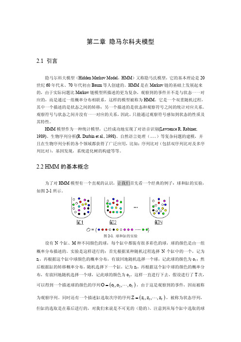
第二章 隐马尔科夫模型2.1 引言隐马尔科夫模型（Hidden Markov Model ，HMM ）又称隐马氏模型，它的基本理论是20世纪60年代末、70年代初由Baum 等人创建的。

HMM 是在Markov 链的基础上发展起来的，由于实际问题比Markov 链模型所描述的更为复杂，观察到的事件并不是与状态一一对应的，而是通过一组概率分布相联系，这样的模型被称为HMM 。

它是一个双重随机过程，其中一个描述的是状态之间的转移；另一个描述的是状态和观察符号之间的统计对应关系。

观察符号与状态之间并没有一一对应的关系，因此，只能通过观察符号感知到状态的性质及其特性。

HMM 模型作为一种统计模型，已经成功地实现了对语音识别(Lawrence R. Rabiner, 1989)、生物序列分析(R. Durbin et al., 1998)、自然语言处理（。

）等复杂问题的建模，并且在生物序列分析的各个领域都获得了广泛应用，比如：序列比对（包括双序列比对及多序列比对），基因发现，系统进化树的构建等等。

2.2 HMM 的基本概念为了对HMM 模型有一个直观的认识，让我们首先看一个经典的例子：球和缸的实验，如图2-1所示。

图2-1. 球和缸的实验设有N 个缸、M 种不同颜色的球，每个缸中都装有很多彩色的球，球的颜色是由一组概率分布描述的。

实验是这样进行的：首先根据某种随机过程选择N 个缸中的一个，记为z 1，再根据这个缸中球颜色的概率分布，有放回地随机选择一个球，记此球的颜色为o 1；然后根据缸的转移概率分布，随机选择下一个缸，记为z 2，再根据这个缸中球的颜色的概率分布，有放回地随机选择一个球，记此球的颜色为o 2。

这样一直进行下去，假设进行了T 次，可以得到一个描述球的颜色的序列()12,,,T O o o o = ，由于这是观察到的事件，因而被称为观察序列。

同时还有一个描述缸选取次序的序列()12,,,T Z z z z = ，被称为状态序列，但缸的选取是在幕后进行的，对我们来说是不可见的（隐的）。

解释聚类模型中的簇标签聚类模型是一种无监督学习算法，用于将数据集中的样本分组成不同的簇。

簇标签是指将每个簇分配一个标签，用于表示该簇的特征或含义。

在本文中，我将详细解释聚类模型中的簇标签，并探讨其在数据分析和机器学习中的应用。

首先，让我们了解一下聚类模型是如何工作的。

聚类算法旨在发现数据集中样本之间的相似性和差异性，并根据这些相似性和差异性将样本分组成不同的簇。

聚类模型通常基于距离或相似度度量来计算样本之间的相似性或差异性。

在聚类过程中，每个样本都被认为是一个多维特征空间中的一个点。

通过计算这些点之间的距离或相似度，我们可以确定它们之间是否属于同一个簇。

根据选择的距离度量和聚类算法，不同类型的数据可以被分配到不同数量和形态各异的簇。

一旦完成了聚类过程，我们需要为每个生成的簇分配一个标签来表示其特征或含义。

这就是所谓的簇标签。

簇标签可以是任何形式的标识符，例如数字、字母、词语或短语。

簇标签的选择应该是基于对数据集和聚类结果的理解和解释。

在选择簇标签时，我们可以根据以下几个因素进行考虑：1. 簇内样本的相似性：在一个簇内，样本之间应该具有相似的特征或属性。

因此，我们可以根据这些特征或属性来为该簇分配一个合适的标签。

2. 簇间样本的差异性：不同簇之间应该有明显不同的特征或属性。

通过比较不同簇之间样本的特征差异，我们可以为每个簇分配一个能够准确反映其差异性和特征的标签。

3. 语义一致性：为了能够更好地理解聚类结果，我们需要选择具有一定语义一致性和可解释性的簇标签。

这意味着选择那些能够准确描述每个聚类结果并与领域知识相符合的标签。

4. 人类可理解性：最终目标是使聚类结果对人来说易于理解和解释。

因此，在选择簇标签时，我们应该考虑人类的认知和理解能力，选择那些能够直观地表示簇的含义和特征的标签。

簇标签在数据分析和机器学习中具有广泛的应用。

以下是一些常见的应用场景：1. 数据理解和可视化：通过为每个簇分配一个标签，我们可以更好地理解数据集中样本之间的相似性和差异性。

markercluster聚合原理摘要：一、MarkerCluster聚合原理简介1.背景介绍2.聚合原理概述二、MarkerCluster核心概念1.标记（Marker）2.标签（Label）3.聚类（Clustering）三、MarkerCluster算法流程1.数据准备2.相似度计算3.聚类划分4.标记生成5.标签分配四、MarkerCluster优缺点分析1.优点2.缺点五、实际应用案例1.文本聚类2.图像聚类3.网络数据聚类六、MarkerCluster在数据挖掘中的应用1.数据降维2.特征提取3.主题发现七、MarkerCluster的未来发展展望1.算法改进2.跨领域应用3.深度学习与MarkerCluster的结合正文：一、MarkerCluster聚合原理简介MarkerCluster聚合原理是一种基于标记和标签的聚类方法。

在众多数据聚类技术中，MarkerCluster脱颖而出，以其独特的聚类思路和良好的聚类效果受到广泛关注。

1.背景介绍随着大数据时代的到来，数据量呈现出爆炸式增长，如何在海量数据中挖掘有价值的信息成为了一项重要任务。

数据聚类作为一种无监督学习方法，可以自动将相似数据组织在一起，从而发现数据之间的内在联系。

在这样的背景下，MarkerCluster应运而生。

2.聚合原理概述MarkerCluster聚合原理基于标记和标签的思想，通过对数据进行相似度计算和聚类划分，实现数据的聚合。

具体来说，它通过计算数据点之间的距离或相似度，将相似的数据点划分为一类，从而实现数据的聚类。

二、MarkerCluster核心概念1.标记（Marker）在MarkerCluster中，标记是用于表示数据点的一种概念。

每个数据点都拥有一个唯一的标记，可以用来区分不同数据点。

2.标签（Label）标签是用于表示标记聚类结果的一种概念。

每个聚类都有一个唯一的标签，可以用来表示聚类的性质和特征。

隐马尔可夫链(Hidden Markov Model, HMM)是一种统计模型，被广泛应用于语音识别、自然语言处理、生物信息学等领域。

在实际应用中，通过解码隐马尔可夫链，可以获得隐藏状态序列，从而推断观测序列的概率分布。

但由于隐马尔可夫链模型的复杂性，传统解法在计算上存在一定的困难。

1. 隐马尔可夫链的常规解法在传统的解法中，针对隐马尔可夫链的解法通常采用经典的Baum-Welch算法和Viterbi算法。

Baum-Welch算法主要用于参数估计，通过迭代的方法对模型的参数进行优化，以使模型能够更好地拟合观测数据。

而Viterbi算法则用于解码，通过动态规划的思想，寻找最可能的隐藏状态序列。

这两种算法在一定程度上能够解决隐马尔可夫链的推断问题，但在实际应用中存在着一些限制。

2. 变分推断的概念变分推断(Variational Inference)是一种近似推断方法，用于解决复杂概率模型中的推断问题。

与传统的精确推断方法相比，变分推断允许以一种近似的方式来推断潜在变量的后验分布。

通过引入一个可调的变分分布，将原始模型的推断问题转化为最小化两个分布之间的差异。

变分推断在处理隐马尔可夫链等复杂模型时具有一定的优势。

3. 变分推断在隐马尔可夫链中的应用近年来，越来越多的研究者开始将变分推断引入到隐马尔可夫链的推断问题中。

通过构建一个合适的变分分布，能够有效地近似隐马尔可夫链的后验分布，从而实现对隐藏状态序列的推断。

在实际应用中，变分推断能够更好地应对隐马尔可夫链模型的复杂性，提高推断的准确性和效率。

4. 变分推断的优势相对于传统的解法，变分推断在处理隐马尔可夫链的推断问题时具有以下优势：- 算法更加灵活和高效。

变分推断允许引入合适的变分分布，从而能够更好地适应不同的模型结构和参数设置，提高了模型的灵活性和推断的效率。

- 结果更加准确和稳定。

通过最小化变分推断分布和真实后验分布之间的差异，能够得到更加准确和稳定的推断结果，提高模型的推断能力。