Adams软件后置处理
- 格式:docx
- 大小:28.64 KB
- 文档页数:3

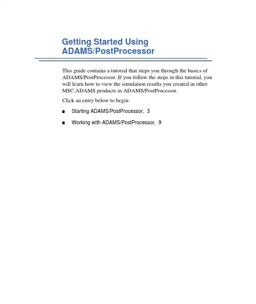
Getting Started UsingADAMS/PostProcessorThis guide contains a tutorial that steps you through the basics of ADAMS/PostProcessor. If you follow the steps in this tutorial, you will learn how to view the simulation results you created in other MSC.ADAMS products in ADAMS/PostProcessor.Click an entry below to begin:■Starting ADAMS/PostProcessor,3■Working with ADAMS/PostProcessor,9Getting Started Using ADAMS/PostProcessor 2CopyrightThe information in this document is furnished for informational use only, may be revised from time to time, and should not be construed as a commitment by MSC.Software Corporation. MSC.Software Corporation assumes no responsibility or liability for any errors or inaccuracies that may appear in this document.Copyright InformationThis document contains proprietary and copyrighted information. MSC.Software Corporation permits licensees of MSC.ADAMS software products to print out or copy this document or portions thereof solely for internal use in connection with the licensed software. No part of this document may be copied for any other purpose or distributed or translated into any other language without the prior written permission of MSC.Software Corporation.Copyright © 2004 MSC.Software Corporation. All rights reserved. Printed in the United States of America. TrademarksADAMS, EASY5, MSC, MSC., MSC.ADAMS, MSC.EASY5, and all product names in the MSC.ADAMS Product Line are trademarks or registered trademarks of MSC.Software Corporation and/or its subsidiaries.NASTRAN is a registered trademark of the National Aeronautics Space Administration. MSC.Nastran is an enhanced proprietary version developed and maintained by MSC.Software Corporation. All other trademarks are the property of their respective owners.Government UseUse, duplication, or disclosure by the U.S. Government is subject to restrictions as set forth in FAR 12.212 (Commercial Computer Software) and DFARS 227.7202 (Commercial Computer Software and Commercial Computer Software Documentation), as applicable.Starting ADAMS/PostProcessorOverviewWe’ve provided a tutorial that steps you through the basics ofADAMS/PostProcessor. If you follow the steps in this tutorial, youwill learn how to view the simulation results you created in otherMSC.ADAMS products in ADAMS/PostProcessor. The sections inthe chapter are:■What You Will Do in the Tutorial, 4■Starting ADAMS/PostProcessor, 4■Loading the Simulation Results, 5The tutorial takes about 20 minutes to complete.Getting Started Using ADAMS/PostProcessor 4Starting ADAMS/PostProcessorWhat You Will Do in the TutorialIn the tutorial, you’ll learn how to:1View reports.2Play an animation of simulation data, including animating the results of a clearance study.3Display simulation results as both xy plots and tables.4View animations and plots simultaneously.Starting ADAMS/PostProcessorYou can run ADAMS/PostProcessor as a stand-alone product or from within other MSC.ADAMS products, such as ADAMS/View, ADAMS/Car, or ADAMS/Engine. The following instructions explain how to start ADAMS/PostProcessor in stand-alone mode. It also explains how to start any add-ons or plugins to ADAMS/PostProcessor. Currently, the only plugin is for ADAMS/Durability.To start ADAMS/PostProcessor stand-alone in UNIX:1At the command prompt, enter the command to start the MSC.ADAMS Toolbar, and then press Enter. The standard command that MSC.Softwareprovides is adams x, where x is the version number, for example, adams2005represents MSC.ADAMS 2005.The MSC.ADAMS Toolbar appears.2Click the ADAMS/PostProcessor tool .For more information on the MSC.ADAMS Toolbar, see the guide, Runningand Configuring MSC.ADAMS on UNIX.To start ADAMS/PostProcessor stand-alone in Windows:■From the Start menu, point to Programs, point to MSC.Software, point to MSC.ADAMS 2005, point to APostProcessor, and then select ADAMS -PostProcessor.For more information on running MSC.ADAMS products from the Startmenu, see the guide, Running MSC.ADAMS on Windows.Getting Started Using ADAMS/PostProcessorStarting ADAMS/PostProcessor5Loading the Simulation ResultsWe’ve provided you with simulation results that you can use to learn the basics of ADAMS/PostProcessor. The simulation results are in two files:■ppt_gs.gra - Graphics file containing information that enablesADAMS/PostProcessor to animate a model of a suspension. It also containstime-dependent data describing the position and orientation of each part in themodel.■ppt_gs.req - Request file containing information that enablesADAMS/PostProcessor to create plots of simulation results. It containsinformation about the various data requested and time history of all the requestvalues.In this tutorial, you import these files through the command file ppt_gs.cmd. The command file also sets up several pages containing animations and plots. In addition, it runs a clearance study as it loads the files.The files are located in the directory /install_dir/ppt/examples, where install_dir is the directory where you installed the MSC.ADAMS products. To get the results into ADAMS/PostProcessor, you need to copy the files to your working directory and import the command file.To copy the files:■In the directory /install_dir/ppt/examples, copy the following files to your working directory:■ppt_gs.cmd■ppt_gs.req■ppt_gs.gra■ppt_gs.html■ppt_gs.pngGetting Started Using ADAMS/PostProcessor 6Starting ADAMS/PostProcessor To import ppt_gs.cmd:1From the File menu, point to Import, and then select Command File.2Right-click the File Name box, and then select Browse.3Use the Open dialog box to find the file ppt_gs.cmd, and then select OK.4In the File Import dialog box, select OK.The command file that you imported into ADAMS/PostProcessor creates several pages containing reports, animations, and plots. It also runs a clearance study.Familiarizing Yourself with ADAMS/PostProcessorADAMS/PostProcessor has four modes:animation, plotting, reports, and 3D plotting (only available with ADAMS/Vibration and ADAMS/Engine data). It switches its modes automatically depending on the contents of the active viewport. For example, the tools in the Main toolbar change if you load an animation or a plot into a viewport.Figure1 on page 7shows the ADAMS/PostProcessor window. The elements shown are common to all modes.Getting Started Using ADAMS/PostProcessorStarting ADAMS/PostProcessor 7Figure 1. ADAMS/PostProcessor WindowThe elements in the ADAMS/PostProcessor window are:■Menu bar - Contains the headings of each menu. ■Main toolbar - Displays commonly used tools for working with animations, plotting results, and reports. It changes depending on whether you are viewinganimations, plots, or reports.■Treeview - Displays a hierarchical list of the models and pages. The tree is especially useful for selecting and identifying objects.■Property editor - Lets you change the properties of selected objects.■Status toolbar - Displays information messages and prompts while you work.■Page - Displays the current page. Each page can display up to six rectangular areas or viewports in which you can place animations and plots.■Viewports - Rectangular areas that display different views of plots, animations, or reports.■Dashboard - Provides functions for controlling animations or plotting results.Status toolbarGetting Started Using ADAMS/PostProcessor 8Starting ADAMS/PostProcessorWorking with ADAMS/PostProcessor OverviewThis chapter steps you through working with three of theADAMS/PostProcessor modes: reports, animations, and plotting:■Displaying Reports, 10■Working with Animations, 10■Working with Plots, 12■Viewing Plots and Animations Simultaneously, 17■The Next Step, 17Getting Started Using ADAMS/PostProcessor 10Working with ADAMS/PostProcessor Displaying ReportsThe first page, which ADAMS/PostProcessor displays by default, is a page p1_report, which displays a report of the pages that the command file you imported created. As you can see from the report, you can use simple HTML tags and bitmapped images to display information about the animations and plots in ADAMS/PostProcessor. You can also display reports of clearance studies. For more information on displaying reports and the HTML tags that ADAMS/PostProcessor supports, see the ADAMS/PostProcessor online help.Working with AnimationsNow you’ll review the animation you loaded with the clearance study results that ADAMS/PostProcessor just performed. You’ll view the animations in different ways, including interactively setting the speed at which ADAMS/PostProcessor runs the animations.Viewing an AnimationThe animation that you will view is stored on the page named p2_clearance.To select the animation page:■In the treeview, select p2_clearance.ADAMS/PostProcessor switches to animation mode and displays the first frame of the animation. All the elements in the dashboard change to those forcontrolling animations. The pull-down menu at the top ofADAMS/PostProcessor to the right of the toolbar also changes to Animation toindicate the current mode.Notice the red and green lines in the animation:■The green line tracks the distance between the right wheel (PART_21) and the steering wheel (PART_10).■The red line tracks the distance between the left wheel (PART_22) and the steering wheel (PART_10).Working with ADAMS/PostProcessor11 To run the animation:■At the top of the dashboard, select the Play tool.Notice that ADAMS/PostProcessor continuously plays the animation. You can also set ADAMS/PostProcessor so that it plays the animation only once or plays the animation forward and then backward.To set the animation to play only once:1On the dashboard, select Animation, if necessary.2Set Loop to Once.Interactively Playing the AnimationTo help you investigate the results of a simulation, you can play animation frames forwards and backwards, rewind to an earlier frame, or play only a portion of the animation. In this tutorial, you’ll interactively play the animation by dragging the animation slider.To interactively play the animation:1To rewind the animation, select the Reset tool.2At the top of the dashboard, drag the slider bar back and forth to watch how the animation plays backwards and forwards at the speed at which you drag the slider.Working with PlotsADAMS/PostProcessor also plots the results of simulations so you can interpret the performance of your design. In this section, you’ll view pages with plots on them, modify the plots, and create your own plots.Viewing Pages of PlotsA page, called p3_plots, already exists that contains several plots that you will view. You’ll first view all the plots and then you’ll quickly zoom in on just one of the plots. Notice that p3_plots in the lower left corner is a plot that ADAMS/PostProcessor has displayed as a table. In the treeview, it is still listed as a plot.To view the plotting page:1In the treeview, select p3_plots.ADAMS/PostProcessor switches to plotting mode and displays the plots.2Click the plot in the upper right corner of the window and, from the Main toolbar,select the Expand View tool.ADAMS/PostProcessor displays only the selected plot.3To return to viewing all the plots, select the Expand View tool again.Working with ADAMS/PostProcessor13Modifying Plotting ObjectsYou can tailor the appearance of plots to help you identify the information in the plot more effectively or to make the plot ready for a presentation. In this section, you’ll turn off the grid lines and change the line style of the curves of one of the plots.Displaying the Table as a PlotBefore you begin to change the look of plots, you’ll change the plot displayed as a table (plot_4) back to being an xy plot.To change the table to a plot:1In the viewport, select plot_4.2In the property editor, clear the selection of Table.Turning Off Grid LinesIn ADAMS/PostProcessor, plots contain primary and secondary grid lines that serve as visual guides for inspecting curves. Primary grid lines appear at all major unit sections. Secondary grid lines appear at specified intervals between the primary grid lines. In this section, you’ll turn off the visibility of the grid lines in one plot. You’ll do this by selecting the plot and then editing its properties in the Property Editor.To turn off primary lines:1Click the border of the plot in the upper right corner.Notice that the viewport border turns red to indicate that you’ve selected it. Inaddition, the treeview highlights the plot. You are now ready to edit the properties of the selected plot.2In the property editor, select Grid.3Clear the selection of Visible.4In the property editor, select the right arrow key to display more tabs.5Select 2nd Grid.6Clear the selection of Visible.Changing Color and Line Style of All CurvesNow you’ll use the treeview to learn how to modify a group of common objects all at once. In this example, you’ll change the line styles of all the curves in the plots on page p3_plots.To change all curves:1To expand the treeview so it displays all plots on the page p3_plots, in the treeview, click the plus sign (+) in front of the page p3_plots.2Now click the plus sign (+) in front of each plot on the page p3_plots to see all the objects in the plots.3In the treeview, hold down the Ctrl key, and select each curve on page p3_plots.4In the property editor, from the Line Style box, select Dash.All the curves change to dashed lines.To reset the filter to show all objects:■Right-click the background of the treeview, point to Type Filter, and then select All.Creating New PlotsYou can also create your own plots as shown in the next steps.Creating a PageBefore you can create a plot, you need to create a page for it.To create a page:■On the Main toolbar, select the New Page tool.Because you are in plotting mode, ADAMS/PostProcessor displays plots onwhich to add data. If you were in animation mode, ADAMS/PostProcessorwould display empty viewports for loading animations.To set the layout of the page so it contains two viewports:■In the Main toolbar, right-click the Page Layout tool stack, and then select .Working with ADAMS/PostProcessor15Adding Data to the PlotNow that you have a new page, you can display some curves on it. In plot mode, the dashboard contains the numeric results of loaded simulation results. It displays the objects, measures, requests, and result sets from ADAMS simulations and any results from clearance studies. The results that you have available depend on the output that you requested from your MSC.ADAMS product. For information on the different results you can generate, see your MSC.ADAMS product online help.In this tutorial, you’ll use requests, which provide standard displacement, velocity, acceleration, or force information that will help you investigate the results of your simulation. Requests also let you define other quantities (such as pressure, work, energy, momentum, and more) that you want generated during a simulation.To add a curve to the plot, select the following from the dashboard:1In the dashboard, in the Request box, select REQ1080 TOE CASTER CAMBER (FRONT).2In the Component box, select X, Y, and Z.3Select Add Curves.4Now add more curves by selecting different data from the dashboard and selecting Add Curves.Surfing Through DataIn the previous section, for each request you selected, ADAMS/PostProcessor added new curves to your plot. You can also plot your data without accumulating curves on your plot. This is called surfing. It is convenient for quickly looking at different data.To quickly add data without creating new curves:1Select the plot on the right.2In the dashboard, select Surf.3Select the data that you’d like to view, as explained earlier.You’ll notice that each time you select data, ADAMS/PostProcessor replaces the existing curves with new curves.Modifying a CurveNot only can you view data in ADAMS/PostProcessor, but you can also change and enhance it. In this tutorial, you’ll change the mathematical expression that creates a curve. To change a curve:1Click a curve on the plot on the left.2At the top of the dashboard, select Math.The dashboard displays the mathematical expressions used to calculate the curve. 3In the Y Expression box, change the mathematical expression, and then select Apply.You can change it in different ways. For example, enter a negative sign(-) in front of the expression to invert the values or multiply the expression by 3.Working with ADAMS/PostProcessor17Viewing Plots and Animations SimultaneouslyYou can place plots and animations together on the same page, and you can also run the animation and see ADAMS/PostProcessor track the corresponding data on the plot as the animation plays.To view plots and animations together:1In the treeview, select the page p4_combined.ADAMS/PostProcessor displays a page containing both animations and plots.2At the top of the dashboard, select the Play tool.ADAMS/PostProcessor plays the animation and displays a line on the plot at the same data point that the animation is displaying.The Next StepYou completed a few of the most common operations in ADAMS/PostProcessor for working with simulation results. Now use the ADAMS/PostProcessor online help as a reference to the many features of ADAMS/PostProcessor.。
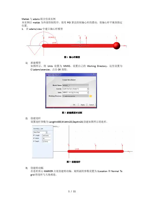
Matlab与adams联合仿真实例本实例以matlab为外部控制程序,使用PID算法控制偏心杆的摆动,使偏心杆平衡到指定位置。
1.在adams/view中建立偏心杆模型图1 偏心杆模型1)新建模型如图所示,将Units设置为MMKS。
设置自己的Working Directory,这里设置为C:\adams\exercise。
点击OK按钮。
图2 新建模型对话框2)创建连杆设置连杆参数为Length=400,Width=20,Depth=20,创建如图所示的连杆。
图3 创建连杆3)创建转动幅在连杆质心MARKER点处创建转动幅,旋转副的参数设置为1Location和Normal To grid将连杆与大地相连。
图4 创建转动幅4)创建球体球体选项设置为Add to part,半径设置为20,单击连杆右侧Marker点,将球体添加到连杆上图5 创建球体5)创建单分量力矩单击Forces>Create a Torque(Single Component)Applied Forces,设置为Space Fixed,Normal to Grid,将Characteristic设置为Constant,勾选Torque并输入0,单击连杆,再点击连杆左侧的Marker点,在连杆上创建一个单分量力矩。
图6 创建单分量力矩2.模型参数设置1)创建状态变量图7 新建状态变量点击图上所示得按钮,弹出创建状态变量对话框,创建输入状态变量Torque,将Name 修改为.MODEL_1.Torque。
图8 新建输入状态变量Torque再分别创建状态变量Angel和Velocity(后面所设计控制系统为角度PID控制,反馈变量为Angel,Velocity为Angel对时间求导,不需要变量Velocity,这里设置Velocity是为了展示多个变量的创建)。
设置Angel的函数AZ(MARKER_3,MARKER_4)*180/PI,Velocity的函数为WZ(MARKER_3,MARKER_4)*180/PI。
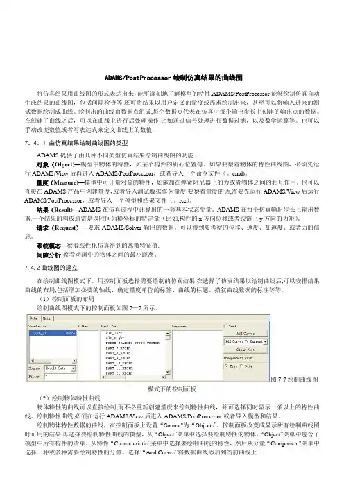
ADAMS/PostProcessor绘制仿真结果的曲线图将仿真结果用曲线图的形式表达出来,能更深刻地了解模型的特性.ADAMS/PostProcessor能够绘制仿真自动生成结果的曲线图,包括间隙检查等,还可将结果以用户定义的量度或需求绘制出来,甚至可以将输入进来的测试数据绘制成曲线。
绘制出的曲线由数据点组成,每个数据点代表在仿真中每个输出步长上创建的输出点的数据。
在创建了曲线之后,可以在曲线上进行后处理操作,比如通过信号处理进行数据过滤,以及数学运算等。
也可以手动改变数值或者写表达式来定义曲线上的数值.7。
4。
1 由仿真结果绘制曲线图的类型ADAMS提供了由几种不同类型仿真结果绘制曲线图的功能.对象(Object)—模型中物体的特性,如某个构件的质心位置等。
如果要察看物体的特性曲线图,必须先运行ADAMS/View后再进入ADAMS/PostProcessor,或者导入一个命令文件(。
cmd)。
量度(Measure)—模型中可计量对象的特性,如施加在弹簧阻尼器上的力或者物体之间的相互作用。
也可以直接在ADAMS产品中创建量度,或者导入测试数据作为量度.要察看量度的话,需要先运行ADAMS/View后运行ADAMS/PostProcessor,或者导入一个模型和结果文件(。
res)。
结果(Result)—ADAMS在仿真过程中计算出的一套基本状态变量。
ADAMS在每个仿真输出步长上输出数据.一个结果的构成通常是以时间为横坐标的特定量(比如,构件的x方向位移或者铰链上y方向的力矩)。
请求(Request)—要求ADAMS/Solver输出的数据。
可以得到要考察的位移、速度、加速度、或者力的信息。
系统模态—察看线性化仿真得到的离散特征值.间隙分析-察看动画中的物体之间的最小距离。
7.4.2曲线图的建立在绘制曲线图模式下,用控制面板选择需要绘制的仿真结果.在选择了仿真结果以绘制曲线后,可以安排结果曲线的布局,包括增加必要的轴线、确定量度单位的标签、曲线的标题、描叙曲线数据的标注等等。
Adams/Vibration后台运行本文主要说明利用Adams/Vibration模块在频域范围内进行后台分析,这在实际工程中有一定的应用。
要完成这一分析流程,需要借助Python编译环境,Python作为一款应用广泛的编程软件,在很多工程仿真软件上都有其拓展应用的身影。
基本步骤:1.利用Adams创建振动分析用的模型,并以Adm方式保存,还需要有控制仿真过程的脚本文件,即Acf文件;2.利用Adams与Python的接口功能定义激励信号,输入通道,输出通道;3.利用Adams与Python的接口功能定义输出,将线性系统的频响特性保存在Xml文件中,同时生成Cmd文件用于Adams后处理;具体执行过程如下:第一,启动cmd命令窗口,并将工作路径指定到相关位置:C:\Users\cnzc8469\Desktop\batch。
点击回车后会产生如下变化,但最关键的是如下文件的生成:这里面关键的设置在Python脚本文件中,需要工程师首先熟悉Python的语法格式以及同Adams相关的API,可以参考帮助下的Testing your model章节,有详细地接口函数说明。
from msc.ADAMS.Vibration.AvActuator import *from msc.ADAMS.Vibration.AvOutputChannel import *from msc.ADAMS.Vibration.AvInputChannel import *from msc.ADAMS.Vibration.AvLinearize import *from msc.ADAMS.Vibration.AvUtils import *from AvPPTCmdExporter import *############################################这一部分相当于Include包含文件功能def message_handler(msg, type, data):"""Message handler for vibration"""if type[0] == "i":print "ADAMS/Vibration Info: %s" % (msg)elif type[0] == "w":print "ADAMS/Vibration Warn: %s" % (msg)else :print "ADAMS/Vibration Error: %s" % (msg)if __name__ == '__main__':# open a log file for logging messageslogFile = open("sla_batch.log", "w")try:# Check out the vibration licensevib_ok = AvAPI.AcquireLicense()if vib_ok:# set message handlerAvAPI().PushMessageHandler(message_handler, [])# 创建激励信号act_vert = AvActuatorSweptSine('SS1', 'Displacement', 5, 0)#创建输入通道,注意相关参数InChVert = AvInputChannelMarker("PadDispInput", 114, "Translational", "Global", "Z", act_vert)inList = [InChVert]# 创建输出通道CVA= AvOutputChannelPredefined("ChassisVertAccl", 105, "Acceleration", "Z") # Measure acceleration at steering rack.TRA= AvOutputChannelPredefined("TieRodAccl", 100, "Acceleration", "X") outList = [CVA, TRA]base_name = "sla_batch"MDI_CPU = os.environ['MDI_CPU']TOPDIR = os.environ['topdir']if MDI_CPU == "win32":if os.path.isdir(TOPDIR) != 0:TOPDIR = os.environ['SHORT_TOPDIR']base_path =TOPDIR+'/vibration/examples/python_batch_analysis/'+base_namemodel = base_path+".adm"acFile = base_path+".acf"#上面两行读取对应模型与脚本控制命令文件mList = []# 创建振动仿真分析参数,如模型名称,频域设定等Model = AvLinearModel(model, inList, outList, acFile, True, base_name, mList) if Model:# set the frequenciesf = AvMakeFrequency(0.1, 250, 500, True)Freq = AvAPI_Matrix(len(f), f)# 计算频响FR = Model.FrequencyResponse(Freq)# 传递函数TF = Model.TransferFunction(Freq)# 将计算结果写入到XML文件中matFile = open(base_name+".xml", "w")writeXMLHeader(matFile)writeMatrixXML(matFile, Freq, "Frequency range" )writeMatrixXML(matFile, FR, "Frequency Response")writeMatrixXML(matFile, TF, "Transfer Function" )writeXMLFooter(matFile)matFile.close()# 生成CMD文件用于后处理中amdModel = AvAMD(model)pptCmdExporter = VibPPTCmdExporter(".sla_basic", base_name+".cmd", amdModel, inList, outList, 0.1, 250.0, 500, True)pptCmdExporter.writeCmdForPPT(base_name)else:logFile.write("Could not produce linear model check execution display for errors.")AvAPI().PopMessageHandler()# 检查口令许可AvAPI.ReleaseLicense()else:logFile.write("Could not get ADAMS/Vibration Solver license")except Exception:formatExceptionInfo(logFile)最后,可以直接打开Adams后处理界面,将生成的CMD文件导入,查看相关信息,如频响等内容。
第7章ADAMS/PostProcessor使用方法本章主要介绍ADAMS/PostProcessor的使用方法,包括ADAMS/PostProcessor的基本操作、输出仿真结果动画、绘制仿真结果曲线图及对曲线图进行处理,最后通过实例介绍ADAMS/PostProcessor的具体用法。
通过本章的学习可以深入了解和具体掌握ADAMS/PostProcessor的基本使用方法,能够结合用户需求灵活地进行仿真计算结果的观察和分析。
7.1ADAMS/PostProcessor简介7.1.1ADAMS/PostProcessor的用途ADAMS/PostProcessor是ADAMS软件的后处理模块,绘制曲线和仿真动画的功能十分强大,利用ADAMS/ PostProcessor可以使用户更清晰地观察其他ADAMS模块(如ADAMS/View,ADAMS/Car或ADAMS/Engine)的仿真结果,也可将所得到的结果转化为动画、表格或者HTML等的形式,能够更确切地反映模型的特性、便于用户对仿真计算的结果进行观察和分析。
ADAMS/PostProcessor在模型的整个设计周期中都发挥着重要的作用,其用途主要包括:1)模型调试在ADAMS/PostProcessor中,用户可选择最佳的观察视角来观察模型的运动,也可向前、向后播放动画,从而有助于对模型进行调试。
也可从模型中分离出单独的柔性部件,以确定模型的变形。
2)试验验证如果需要验证模型的有效性,可输入测试数据并以坐标曲线图的形式表达出来,然后将其与ADAMS仿真结果绘于同一坐标曲线图中进行对比,并可以在曲线图上进行数学操作和统计分析。
3)设计方案改进在ADAMS/PostProcessor中,可在图表上比较两种以上的仿真结果,从中选择出合理的设计方案。
另外,可通过单击鼠标操作,更新绘图结果。
如果要加速仿真结果的可视化过程,可对模型进行多种变化。
也可以进行干涉检验,并生成一份关于每帧动画中构件之间最短距离的报告,帮助改进设计。
关于多学科 - MD 方案MSC.Adams 2010是集建模、求解、可视化技术于一体的虚拟样机软件,是世界上目前使用范围最广、最负盛名的机械系统仿真分析软件。
ADAMS全仿真软件包是一个功能强大的建模和仿真环境,它可以对任何机械系统进行建模、仿真、细化及优化设计,应用范围从汽车、火车、航空航天器一直到盒式录像机等。
使用这套软件可以产生复杂机械系统的虚拟样机,真实地仿真其运动过程,并且可以迅速地分析和比较多种参数方案,直至获得优化的工作性能,从而大大减少了昂贵的物理样机制造及试验次数,提高了产品设计质量,大幅度地缩短产品研制周期和费用。
ADAMS 软件将强大的分析求解功能与使用方便的用户界面相结合,使该软件使用起来既直观又方便,还可用户专门化。
ADAMS软件的特点如下:-利用交互式图形环境和零件库、约束库、力库建立机械系统三维参数化模型。
-分析类型包括运动学、静力学和准静力学分析,以及线性和非线性动力学分析,包含刚体和柔性体分析。
-具有先进的数值分析技术和强有力的求解器,使求解快速、准确。
-具有组装、分析和动态显示不同模型或同一个模型在某一个过程变化的能力,提供多种“虚拟样机”方案。
-具有一个强大的函数库供用户自定义力和运动发生器。
-具有开放式结构,允许用户集成自己的子程序。
-自动输出位移、速度、加速度和反作用力曲线,仿真结果显示为动画和曲线图形。
-可预测机械系统的性能、运动范围、碰撞、包装、峰值载荷以及计算有限元的输入载荷。
-支持同大多数CAD、FEA和控制设计软件包之间的双向通讯。
ADAMS软件可以广泛应用于航空航天、汽车工程、铁路车辆及装备、工业机械、工程机械等领域。
MSC MD ADAMS 2007 R3!Adams(Automatic Dynamic Analysis of Mechanical System)软件是美国MDI(Mechanical Dynamics Inc.)公司(现已经并入美国MSC公司)开发的机械系统动力学仿真分析软件,在全球占有率最高。
Adams柔性体仿真后查看应力应变首先说明,如果想查看柔性体应力计应变,则mnf文件中必须包含模态应力及应变信息。
下面是我建立的模型。
一个简单的四连杆机构,连杆是柔性体。
进行仿真后进入后处理界面。
首先在ADAMS/View中加载ADAMS/Durability模块,这是柔性体后处理(针对应力及应变的后处理)画曲线和观察动画的前提。
(1)画曲线通过以下路径“Tool-->>Plugin Manager”,在对话框中“Load”一栏对应的ADAMS/Durability打勾。
Step1 查看仿真过程应力及应变最大值以及相应的节点号,以便于下面输出曲线时选择相应的节点。
在主菜单Durability一栏下选择Hot Spots Table,出现Hot Spots Information 对话框,通过此对话框,可以得出得到在仿真过程中各个节点的最大应力。
下图显示仿真过程中最大mises应力。
Step2 进入后处理模块ADAMS/Postprocessor在主菜单Durability一栏下选择Nodal Plot,出现以下对话框。
在Flexible Body 一栏选择柔性体名称,在Select Node List一栏输入想要查看的节点编号,选择Stress或Strain等相关选项,点击确定。
Step3 在窗口区,鼠标右键选择load plot进入画曲线窗口。
在Source选项中选择“Result Sets”,result set里面选择“**_STRESS”,进一步往下选择所需要的输出即可以画曲线了。
如上图所示则画出了我建立的模型中node_371的Mises应力时间曲线。
见下图(2)观察动画功能在加载ADAMS/Durability模块后在窗口区右键选择Load Animation进入动画现实界面。
在下端Contour Plots 选项卡下选择“Contour Plot Type”选项,根据需要选择Deformation (变形)或者Von Mises Stress(米塞斯应力)等等。
【Adams应用教程】第7章ADAMSPostProcessor第7章 ADAMS/PostProcessor使用方法本章主要介绍ADAMS/PostProcessor的使用方法,包括ADAMS/PostProcessor的基本操作、输出仿真结果动画、绘制仿真结果曲线图及对曲线图进行处理,最后通过实例介绍ADAMS/ PostProcessor的具体用法。
通过本章的学习可以深入了解和具体掌握ADAMS/ PostProcessor的基本使用方法,能够结合用户需求灵活地进行仿真计算结果的观察和分析。
7.1 ADAMS/PostProcessor简介7.1.1 ADAMS/PostProcessor的用途ADAMS/ PostProcessor是ADAMS软件的后处理模块,绘制曲线和仿真动画的功能十分强大,利用ADAMS/ PostProcessor可以使用户更清晰地观察其他ADAMS模块(如ADAMS/ View, ADAMS/ Car 或ADAMS/ Engine)的仿真结果,也可将所得到的结果转化为动画、表格或者HTML等的形式,能够更确切地反映模型的特性、便于用户对仿真计算的结果进行观察和分析。
ADAMS/PostProcessor在模型的整个设计周期中都发挥着重要的作用,其用途主要包括:(1)模型调试在ADAMS/ PostProcessor中,用户可选择最佳的观察视角来观察模型的运动,也可向前、向后播放动画,从而有助于对模型进行调试。
也可从模型中分离出单独的柔性部件,以确定模型的变形。
(2)试验验证如果需要验证模型的有效性,可输入测试数据并以坐标曲线图的形式表达出来,然后将其与ADAMS仿真结果绘于同一坐标曲线图中进行对比,并可以在曲线图上进行数学操作和统计分析。
(3)设计方案改进在ADAMS/PostProcessor中,可在图表上比较两种以上的仿真结果,从中选择出合理的设计方案。
另外,可通过单击鼠标操作,更新绘图结果。
Adams后处理中测量曲线数据的查看与导出
作者:Simwe 来源:MSC发布时间:2012-05-29 【收藏】【打印】复制连接【大中小】我来说两句:(1) 逛逛论坛
你知道可以以列表的方式查看Adams/PostProcessor中显示的曲线图吗?另外,你可以将一个曲线以数据表的形式导出,也就是说,你能够利用曲线绘图来分类或创建用户自
定义的输出文件。
1.Adams/PostProcessor中利用数据列表方式显示测量曲线
左键选择一个曲线绘图边框,注意不要点击在曲线、图例或坐标轴上。
另一个方法是可以在Adams/Postprocessor左侧窗口的模型树中选择对应的曲线绘图,在这个过程中可能需要点击一个page前的+号以将page中的内容扩展开显示对应的曲线绘图。
当选择了一个曲线绘图后,注意在窗口左下角的属性编辑窗口中的Table复选框。
选择Table复选框后对应的属性编辑窗口将变为观察图表显示的控制窗口。
在视窗中原来的曲线绘图变为了HTML格式的图表数据。
下图例子中显示了单摆的X向和Y向位移。
2.Adams/PostProcessor中曲线数据导出方式
在Adams/PostProcessor中,导出数据有三种方式:Numeric Data,Spreadsheet 和Table。
Numeric Data和Spreadsheet方式导出数据会导出整个结果集中包含的数据,Table方式导出数据只会导出在你所选择的曲线视图中显示的曲线数据。
例如,如果整个仿真时间为2秒,那么Numeric Data,Spreadsheet方式会导出完整的2秒钟内所有的数据点;那么如果你只想导出1秒钟的数据,那么你可以设定坐标横范围为0至1秒,如下
图所示,然后利用Table方式导出数据。
File->Export->Table弹出对话框,在File Name中指定文件名称,将以后缀名".Tab"输出该文件,Plot域中指定那组数据需要输出;你可以直接输入曲线绘图的名称或通过Pick/Browse/Guess工具来找到对应的曲线绘图。
另外有两种数据格式供选择:spreadsheet和HTML格式。
在spreadsheet格式中,每一列数据是通过Tab字符分隔开,模型的名称及每列的标签都以双引号的字符串形式包含在输出文件中。
大部分spreadsheet格式数据可以直接读取,当你导入这些数据报错时,你可以去编辑或删除标
签行。
我们经常需要将adams中的图像数据或轨迹数据导入到matlab进行分析,关于测量曲线数据和轨迹数据的导出方法如下:
1.测量曲线数据的导出
我常用的方法是在postprocessor中,file-export-numeric data,然后以“*.txt”的形式输入文件名,并在result data中browser出想要的数据,点OK。
这样就将图像的x,y的数据以txt 的形式输出。
当然也可以在输入文件名时不加txt后缀,这样生成的文件没有后缀名,只是二进制数据,可以用excel打开,并保存为.xls的格式。
后面会解释要保存为.txt的格式,而不是保存为excel的格式。
2.轨迹数据的导出
我还没发现怎么在postprocesor中找到轨迹曲线的数据,只有在view界面下导出数据了。
利用create trace spline 生成轨迹曲线后,在轨迹曲线上右击-modify-value后的省略号-write,然后以“*.txt”的形式输入文件名,OK。
当曲线和轨迹数据导出后,就可以将其导入到matlab中进行分析。
在网上找到了很多中方法。
1、其中有一种是将.xls格式的文件导入到matlab中的方法,也是很常用的方法,可是我按
照网上的方法使用后出现了matlab XLS File contains unicode text which is not yet
supported的错误,网上的解释说是因为matlab与wps兼容性不好的缘故,我用的是wps 的表格生成的.xls文件,因此这个方法就不行了。
2、如果直接读取txt文件,发现多处了好多无用的数据,也未找到解决方法。
3、在matlab下,用file-import data,打开.txt文件,并选出自己需要的数据存入某个变量。
这里可以自动去掉文件中的字符,只保留数字。
我感觉这种方法导入数据还是挺快的。
导入后就可以直接对生成的变量进行操作以对数据进行分析了。
•c++编程遇到问题总结
•adams的逆向分析。