模拟退火算法解决路径优化 的源代码
- 格式:doc
- 大小:29.50 KB
- 文档页数:11
使用matlab实现模拟退火算法标题:使用MATLAB实现模拟退火算法:优化问题的全局搜索方法引言:模拟退火算法(Simulated Annealing)是一种经典的全局优化算法,常用于解决各种实际问题,如组合优化、参数优化、图形分割等。
本文将详细介绍如何使用MATLAB实现模拟退火算法,并介绍其原理、步骤以及代码实现。
1. 模拟退火算法简介模拟退火算法借鉴了金属退火的物理过程,在解空间中进行随机搜索,用于找到全局最优解。
其核心思想是通过接受一定概率的劣解,避免陷入局部极小值,从而实现全局优化。
2. 模拟退火算法步骤2.1 初始参数设置在使用MATLAB实现模拟退火算法之前,我们需要配置一些初始参数,包括起始温度、终止温度、温度衰减系数等。
这些参数的合理设定对算法的效果至关重要。
2.2 初始解的生成在模拟退火算法中,我们需要随机生成一个初始解,作为搜索的起点。
这个初始解可以是随机生成的,也可以是根据问题本身的特性生成的。
2.3 判定条件模拟退火算法需要一个判定条件来决定是否接受新解。
通常我们使用目标函数值的差异来评估新解的优劣。
如果新解更优,则接受;否则,按照一定概率接受。
2.4 温度更新模拟退火算法中最重要的一步是对温度的更新。
温度越高,接受劣解的概率就越大,随着迭代的进行,温度逐渐降低,最终达到终止温度。
2.5 迭代过程在每次迭代中,我们通过随机生成邻近解,计算其目标函数值,并根据判定条件决定是否接受。
同时,根据温度更新的规则调整温度。
迭代过程中,不断更新当前的最优解。
3. MATLAB实现模拟退火算法在MATLAB中,我们可以通过编写函数或使用内置函数来实现模拟退火算法。
具体的实现方法取决于问题的复杂度和求解的要求。
我们需要确保代码的可读性和可复用性。
4. 示例案例:TSP问题求解为了演示模拟退火算法的实际应用,我们将以旅行商问题(Traveling Salesman Problem,TSP)为例进行求解。
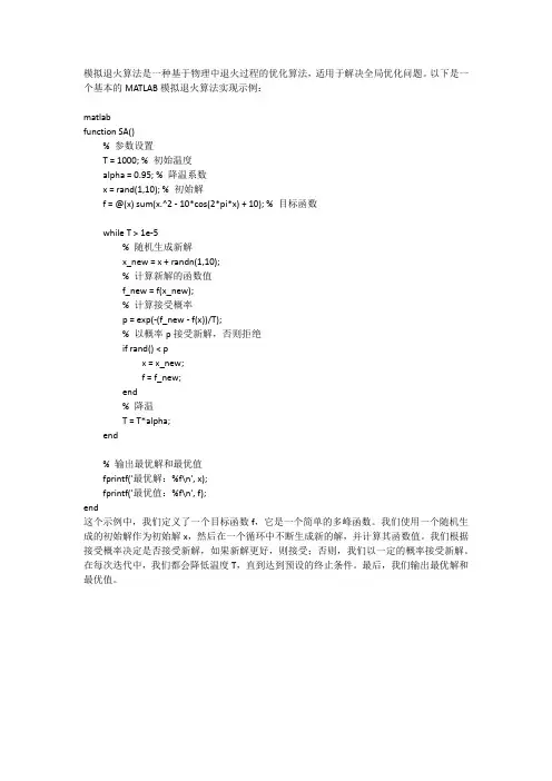
模拟退火算法是一种基于物理中退火过程的优化算法,适用于解决全局优化问题。
以下是一个基本的MATLAB模拟退火算法实现示例:
matlab
function SA()
% 参数设置
T = 1000; % 初始温度
alpha = 0.95; % 降温系数
x = rand(1,10); % 初始解
f = @(x) sum(x.^2 - 10*cos(2*pi*x) + 10); % 目标函数
while T > 1e-5
% 随机生成新解
x_new = x + randn(1,10);
% 计算新解的函数值
f_new = f(x_new);
% 计算接受概率
p = exp(-(f_new - f(x))/T);
% 以概率p接受新解,否则拒绝
if rand() < p
x = x_new;
f = f_new;
end
% 降温
T = T*alpha;
end
% 输出最优解和最优值
fprintf('最优解:%f\n', x);
fprintf('最优值:%f\n', f);
end
这个示例中,我们定义了一个目标函数f,它是一个简单的多峰函数。
我们使用一个随机生成的初始解作为初始解x,然后在一个循环中不断生成新的解,并计算其函数值。
我们根据接受概率决定是否接受新解,如果新解更好,则接受;否则,我们以一定的概率接受新解。
在每次迭代中,我们都会降低温度T,直到达到预设的终止条件。
最后,我们输出最优解和最优值。
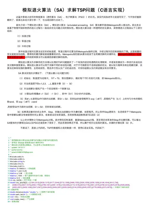
模拟退⽕算法(SA)求解TSP问题(C语⾔实现) 这篇⽂章是之前写的智能算法(遗传算法(GA)、粒⼦群算法(PSO))的补充。
其实代码我⽼早之前就写完了,今天恰好重新翻到了,就拿出来给⼤家分享⼀下,也当是回顾与总结了。
⾸先介绍⼀下模拟退⽕算法(SA)。
模拟退⽕算法(simulated annealing,SA)算法最早是由Metropolis等⼈提出的。
其出发点是基于物理中固体物质的退⽕过程与⼀般组合优化问题之间的相似性。
模拟退⽕算法是⼀种通⽤的优化算法,其物理退⽕过程由以下三部分组成: (1)加温过程 (2)等温过程 (3)冷却过程 其中加温过程对应算法设定的初始温度,等温过程对应算法的Metropolis抽样过程,冷却过程对应控制参数的下降。
这⾥能量的变化就是⽬标函数,要得到的最优解就是能量最低状态。
Metropolis准则是SA算法收敛于全局最优解的关键所在,Metropolis准则以⼀定的概率接受恶化解,这样就使得算法可以跳离局部最优解的陷阱。
模拟退⽕算法为求解传统⽅法难以处理的TSP问题提供了⼀个有效的途径和通⽤的处理框架,并逐渐发展成为⼀种迭代⾃适应启发式概率搜索算法。
模拟退⽕算法可以⽤于求解不同的⾮线性问题,对于不可微甚⾄不连续函数的优化,能以较⼤概率求得全局最优解,该算法还具有较强的鲁棒性、全局收敛性、隐含并⾏性以及⼴泛的适应性,对⽬标函数以及约束函数没有任何要求。
SA 算法实现的步骤如下:(下⾯以最⼩化问题为例) (1)初始化:取温度T0⾜够⼤,令T = T0,取任意解S1,确定每个T时的迭代次数,即 Metropolis链长L。
(2)对当前温度T和k=1,2,3,...,L,重复步骤(3)~(6) (3)对当前解S1随机产⽣⼀个扰动得到⼀个新解 S2. (4)计算S2的增量df = f(S2) - f(S1),其中f(S1)为S1的代价函数。
(5)若df < 0,接受S2作为新的当前解,即S1 = S2;否则S2的接受概率为 exp(-df/T),即随机产⽣(0,1)上的均匀分布的随机数rand,若 exp(-df/T)>rand,则接受S2作为新的当前解,S1 = S2;否则保留当前解。
c语言编写的模拟退火算法的代码以下是一个简单的C语言编写的模拟退火算法的代码示例: c.#include <stdio.h>。
#include <math.h>。
#include <stdlib.h>。
#include <time.h>。
#define N 100 // 待优化参数的个数。
#define T_INITIAL 100.0 // 初始温度。
#define T_FINAL 0.1 // 最终温度。
#define ALPHA 0.9 // 降温速率。
// 计算当前解的能量。
double calculateEnergy(double solution[]) {。
// 这里可以根据具体问题来定义能量的计算方式。
// 以下是一个简单的示例,假设能量为各参数的平方和。
double energy = 0.0;for (int i = 0; i < N; i++) {。
energy += solution[i] solution[i];}。
return energy;}。
// 生成新的解。
void generateNewSolution(double currentSolution[], double newSolution[], double T) {。
// 这里可以根据具体问题来定义如何生成新解。
// 以下是一个简单的示例,假设每个参数在当前解的基础上增加一个随机值。
for (int i = 0; i < N; i++) {。
newSolution[i] = currentSolution[i] + (double)rand() / RAND_MAX T;}。
}。
// 模拟退火算法。
void simulatedAnnealing() {。
double currentSolution[N]; // 当前解。
double newSolution[N]; // 新的解。
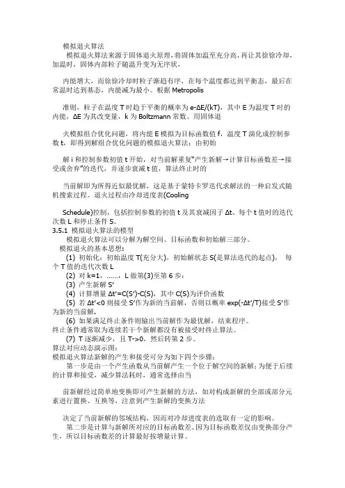
模拟退火算法模拟退火算法是一种通用的随机搜索算法,是局部搜索算法的扩展。
它的思想是再1953年由metropolis提出来的,到1983年由kirkpatrick等人成功地应用在组合优化问题中。
模拟退火算法来源于固体退火原理,将固体加温至充分高,再让其徐徐冷却,加温时,固体内部粒子随温升变为无序状,内能增大,而徐徐冷却时粒子渐趋有序,在每个温度都达到平衡态,最后在常温时达到基态,内能减为最小。
根据Metropolis准则,粒子在温度T时趋于平衡的概率为e-ΔE/(kT),其中E为温度T时的内能,ΔE为其改变量,k为Boltzmann常数。
用固体退火模拟组合优化问题,将内能E模拟为目标函数值f,温度T演化成控制参数t,即得到解组合优化问题的模拟退火算法:由初始解i和控制参数初值t开始,对当前解重复“产生新解→计算目标函数差→接受或舍弃”的迭代,并逐步衰减t值,算法终止时的当前解即为所得近似最优解,这是基于蒙特卡罗迭代求解法的一种启发式随机搜索过程。
退火过程由冷却进度表(Cooling Schedule)控制,包括控制参数的初值t及其衰减因子Δt、每个t值时的迭代次数L和停止条件S。
模拟退火算法新解的产生和接受可分为如下四个步骤:第一步是由一个产生函数从当前解产生一个位于解空间的新解;为便于后续的计算和接受,减少算法耗时,通常选择由当前新解经过简单地变换即可产生新解的方法,如对构成新解的全部或部分元素进行置换、互换等,注意到产生新解的变换方法决定了当前新解的邻域结构,因而对冷却进度表的选取有一定的影响。
第二步是计算与新解所对应的目标函数差。
因为目标函数差仅由变换部分产生,所以目标函数差的计算最好按增量计算。
事实表明,对大多数应用而言,这是计算目标函数差的最快方法。
第三步是判断新解是否被接受,判断的依据是一个接受准则,最常用的接受准则是Metropo1is准则: 若Δt′<0则接受S′作为新的当前解S,否则以概率exp(-Δt′/T)接受S′作为新的当前解S。
pyomo 模拟退火解方程
Pyomo是一个用于建模和求解数学优化问题的Python库,而模
拟退火是一种全局优化算法,通常用于求解复杂的非线性、非凸优
化问题。
要使用Pyomo进行模拟退火来解方程,你可以按照以下步
骤进行:
1. 定义优化模型,首先,你需要使用Pyomo来定义你的优化模型。
这包括定义决策变量、约束条件和优化目标函数。
在这个步骤中,你需要考虑如何将你的方程转化为数学模型的形式。
2. 配置模拟退火算法,Pyomo提供了一些优化算法的接口,包
括模拟退火算法。
你需要配置模拟退火算法的参数,比如初始温度、降温速度等。
这些参数的选择对算法的收敛性和效率有很大影响。
3. 求解优化问题,一旦你的模型和算法都配置好了,你可以使
用Pyomo来求解优化问题。
Pyomo会调用模拟退火算法来尝试找到
方程的最优解。
需要注意的是,将方程转化为优化模型的过程可能会比较复杂,特别是对于非线性方程。
你需要仔细考虑如何将方程的约束条件和
目标函数转化为优化模型的约束条件和目标函数。
此外,模拟退火算法通常用于全局优化,对于特定的方程可能存在更适合的优化算法,你需要权衡选择合适的算法。
总之,使用Pyomo的模拟退火算法来解方程是可行的,但需要仔细思考如何建立数学模型,并对算法的参数进行合适的调整。
希望这些信息能够帮助你开始使用Pyomo进行模拟退火来解方程。
如何在Matlab中进行模拟退火算法的优化模拟退火算法是一种用于求解复杂问题的全局优化算法。
在Matlab中,我们可以利用其强大的数值计算和优化工具箱来实现模拟退火算法的优化。
本文将介绍如何在Matlab中进行模拟退火算法的优化,并通过一个实际的案例来演示其应用。
一、模拟退火算法简介模拟退火算法是一种启发式的全局优化算法,模拟了固体物体在退火过程中的特性。
其基本原理是通过模拟固体退火过程,逐渐降低系统能量,从而找到全局最优解。
在模拟退火算法中,由于退火过程中存在较高的温度,使算法有机会跳出局部极小值点,因此能够在搜索空间中全面地寻找最优解。
二、Matlab中的模拟退火算法优化函数Matlab提供了优化工具箱,在其中包含了一系列优化函数,其中包括模拟退火算法。
我们可以使用"simulannealbnd"函数来在Matlab中实现模拟退火算法的优化。
三、案例演示:函数最优化假设我们要求解以下函数的最小值:f(x) = x^2 + sin(5x)我们可以使用Matlab中的模拟退火算法优化函数来找到该函数的全局最小值。
1. 定义目标函数首先,我们需要在Matlab中定义目标函数:function y = myfunc(x)y = x.^2 + sin(5*x);2. 编写优化代码接下来,我们可以编写优化代码,利用"simulannealbnd"函数进行模拟退火算法的优化:options = saoptimset('Display','iter','TolFun',1e-6);[x,fval] = simulannealbnd(@myfunc, [-10,10],[],[],options);在上述代码中,"options"用于设置优化选项,"@myfunc"是要优化的目标函数,[-10,10]为变量的取值范围,[]表示无约束条件。
模拟退火算法多目标优化代码1模拟退火算法介绍模拟退火算法(Simulated Annealing)是一种优化算法。
该算法借鉴了冶金学中的物理过程“退火”原理,将物质加热到一定温度时,分子运动剧烈,容易跳出能量低的局部最优解,从而找到全局最优解。
模拟退火算法应用物理过程中的思想,通过引入随机性,避免优化算法陷入局部最优解。
2模拟退火算法流程模拟退火算法流程如下:1.初始化状态:随机生成一个初始解,2.设定初温:设定一个初始温度,一般温度初始值为1或者10。
3.迭代搜索:在当前温度下进行迭代搜索,每次随机生成一个新解,并计算新解与当前解的差距,如果新解优于当前解,则接受新解,否则以一定概率接受新解;4.降温:根据一定的降温策略降低温度,一般采用指数降温策略,即每次降低固定的降温速率。
5.终止条件:当达到停止温度或解的变化非常微小,从而收敛到全局最优解,算法结束。
3模拟退火算法多目标优化问题模拟退火算法适用于解决单目标函数优化问题,然而在实际生活中,很多问题往往涉及到多目标的优化问题。
多目标优化问题的关键在于如何权衡不同目标之间的矛盾,寻找最优解是一个非常困难的问题。
4模拟退火算法多目标优化思路对于多目标优化问题,模拟退火算法的关键在于设计合适的评价函数和决策方法。
1.评价函数设计为了解决多目标优化问题,需要使用评价函数来评价每一个解的优劣。
评价函数应包含多个优化目标,并考虑到各个目标之间的权衡关系。
2.决策方法设计在模拟退火算法中,决策方法用于选择新解或保留当前解。
针对多目标优化问题,应该采用Pareto最优解的思想,即选择那些不能被其他解支配的解。
5模拟退火算法多目标优化代码以下是模拟退火算法多目标优化的Python代码示例:```def simulated_annealing_multi_obj(eval_func,init_state, T=1,alpha=0.99,stopping_T=1e-8,stopping_iter=1000): """eval_func:多目标评价函数init_state:初始化状态T:初始温度alpha:降温速率stopping_T:停止温度stopping_iter:停止迭代次数"""state=init_stateC=[1,1,1]#目标函数的加权系数k=0best_state=statebest_eval=eval_func(best_state)while T>=stopping_T and k<stopping_iter:k+=1#随机生成新解new_state=generate_new_state(state)#计算新解的多目标函数值new_eval=eval_func(new_state)#判断新解是否优于当前解if is_pareto_optimal(new_eval,best_eval,C):best_state=new_statebest_eval=new_evalstate=new_stateelse:delta_eval=C[0]*(new_eval[0]-best_eval[0])**2+C[1]*(new_eval[1]-best_eval[1])**2 +C[2]*(new_eval[2]-best_eval[2])**2p=np.exp(-delta_eval/T)if random.random()<p:state=new_state#降温T*=alphareturn best_state,best_eval```6总结在实际的应用场景中,往往需要解决多目标的优化问题。
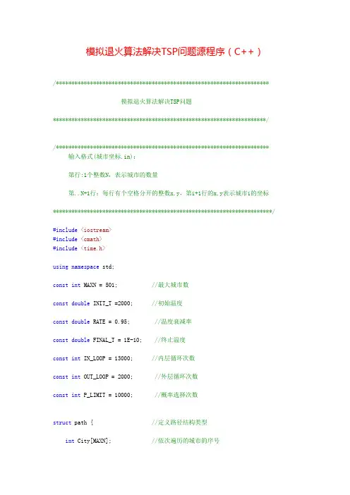
模拟退火算法解决TSP问题源程序(C++)/*********************************************************************模拟退火算法解决TSP问题*********************************************************************//********************************************************************* 输入格式(城市坐标.in):第行:1个整数N,表示城市的数量第..N+1行:每行有个空格分开的整数x,y,第i+1行的x,y表示城市i的坐标***********************************************************************/#include<iostream>#include<cmath>#include<time.h>using namespace std;const int MAXN = 501; //最大城市数const double INIT_T =2000; //初始温度const double RATE = 0.95; //温度衰减率const double FINAL_T = 1E-10; //终止温度const int IN_LOOP = 13000; //内层循环次数const int OUT_LOOP = 2000; //外层循环次数const int P_LIMIT = 10000; //概率选择次数struct path { //定义路径结构类型int City[MAXN]; //依次遍历的城市的序号double Length; //所有城市的路径总长度};int N; //城市数量double D[MAXN][MAXN]; //任意两个城市之间的距离path bestpath; //最优的遍历路径inline double dist(int x1, int y1, int x2, int y2) //计算两点之间的距离{return sqrt(double((x2-x1)*(x2-x1)+(y2-y1)*(y2-y1)));}inline double totaldist(path p) //计算遍历路径P的总长度{int i;double cost = 0;for (i=1; i<N; i++){cost += D[p.City[i]][p.City[i+1]];}cost += D[p.City[1]][p.City[N]];return cost;}void init() //读入数据,并初始化{int C[MAXN][2]; //城市的坐标int i, j;freopen("城市坐标.in", "r", stdin);//freopen("结果输出.out", "w", stdout);scanf("%d", &N);for (i=1; i<=N; i++)scanf("%d%d", &C[i][0], &C[i][1]);for (i=1; i<N; i++) //计算任意两个城市之间的路径长度for (j=i+1; j<=N; j++){D[i][j] = D[j][i] = dist(C[i][0], C[i][1], C[j][0], C[j][1]); }for (i=1; i<=N; i++) //最优解的初始状态bestpath.City[i] = i;bestpath.Length = totaldist(bestpath);srand((unsigned)time(NULL));}/************************************************************产生新路径方法*************************************************************/path getnext(path p) //新解产生函数{int x, y;path ret;ret = p;do {x = rand() % N + 1;y = rand() % N + 1;}while(x == y);swap(ret.City[x], ret.City[y]); //交换两城市之间位置顺序ret.Length = totaldist(ret);return ret;}/****************************************************************退火和降温过程******************************************************************/ void sa(){double T; //温度path newpath, curpath; //当前路径和新路径int i, P_t=0, A_t=0;double delta;T = INIT_T; //赋值初始温度curpath = bestpath;while(true){for (i=1; i<=IN_LOOP; i++){newpath = getnext(curpath); //获取新路径delta = newpath.Length - curpath.Length;if (delta < 0.0){curpath = newpath;P_t = 0;A_t = 0;}else{double rnd = rand()%10000 /10000.0;double p = exp(-delta/T);if (p > rnd)curpath = newpath;P_t++;}if (P_t >=P_LIMIT){A_t++;break;}}if (curpath.Length<bestpath.Length)bestpath = curpath;if ( A_t >= OUT_LOOP || T < FINAL_T) break;T = T * RATE; //降温}}/****************************************************************程序主函数******************************************************************/ int main(){init();printf("初始路径长度: %.4f\n", bestpath.Length);for(int i=0;i<N;){printf(" %d->", bestpath.City[++i]);}printf(" %d", bestpath.City[1]);printf("\n");sa();printf("最优路径长度: %.4f\n", bestpath.Length);for(int j=0;j<N;){printf(" %d->", bestpath.City[++j]);}printf(" %d", bestpath.City[1]);printf("\n");return 0;}城市坐标示例:输出结果示例:。
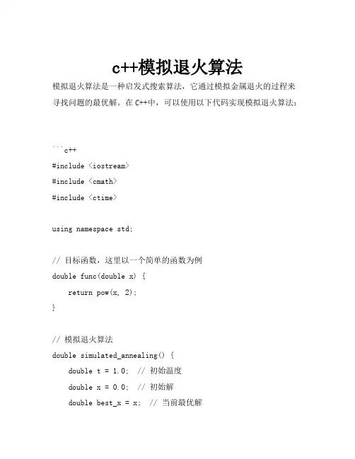
c++模拟退火算法模拟退火算法是一种启发式搜索算法,它通过模拟金属退火的过程来寻找问题的最优解。
在C++中,可以使用以下代码实现模拟退火算法:```c++#include <iostream>#include <cmath>#include <ctime>using namespace std;// 目标函数,这里以一个简单的函数为例double func(double x) {return pow(x, 2);}// 模拟退火算法double simulated_annealing() {double t = 1.0; // 初始温度double x = 0.0; // 初始解double best_x = x; // 当前最优解double best_f = func(x); // 当前最优函数值double step = 1.0; // 初始步长double alpha = 0.95; // 降温系数double f; // 当前函数值double x_new; // 新解int count = 0; // 计数器while (t > 1e-5) {// 在当前解附近随机产生新解x_new = x + step * (rand() % 2 - 0.5);f = func(x_new);// 如果新解更好,则接受新解if (f < best_f) {best_f = f;best_x = x_new;x = x_new;} else {// 如果新解不如当前解,则以一定的概率接受新解 if (rand() % 100 < 50) {x = x_new;}}// 降温t *= alpha;step /= 10;count++;}cout << "最优解: " << best_x << endl;cout << "最优函数值: " << best_f << endl;cout << "迭代次数: " << count << endl;return best_f;}int main() {srand(time(NULL)); // 初始化随机数种子simulated_annealing(); // 运行模拟退火算法return 0;}```在这个例子中,我们使用一个简单的二次函数作为目标函数。
python 模拟退火解方程模拟退火是一种启发式搜索算法,可以用于解决优化问题,例如求解非线性方程组。
以下是使用Python实现模拟退火解方程的示例代码:```pythonimport numpy as npdef simulated_annealing(func, init_state, init_temp, alpha, min_temp, max_iter):"""模拟退火算法:param func: 目标函数:param init_state: 初始状态:param init_temp: 初始温度:param alpha: 降温系数:param min_temp: 最小温度:param max_iter: 最大迭代次数:return: 最佳状态和最佳函数值"""state = init_statetemp = init_tempbest_state = statebest_func_val = func(state)for i in range(max_iter):neighbor = state + (-1, 1) 产生一个邻近状态delta = func(neighbor) - func(state) 计算状态变化导致的函数值变化if delta < 0 or () < (-delta / temp): Metropolis准则state = neighborif func(state) < best_func_val: 更新最佳状态和函数值best_state = statebest_func_val = func(state)temp = max(temp alpha, min_temp) 降温return best_state, best_func_val```使用示例:```pythonfunc = lambda x: (x - 2) 2 目标函数为二次函数,最小值为0,位于x=2处init_state = 0 初始状态为0init_temp = 100 初始温度为100alpha = 降温系数为min_temp = 最小温度为max_iter = 1000 最大迭代次数为1000次best_x, best_val = simulated_annealing(func, init_state, init_temp, alpha, min_temp, max_iter)print("最佳解:x={}, f(x)={}".format(best_x, best_val)) 输出最佳解和对应的函数值```。
车间调度是生产制造过程中非常重要的一个环节,它涉及到原材料的供给、生产设备的利用以及人员的安排,对于提高生产效率和降低成本具有重要意义。
在实际生产中,由于各种因素的不确定性,车间调度问题往往变得复杂而困难。
为了解决这一问题,人们开发了各种车间调度算法,其中模拟退火算法是一种比较有效的方法之一。
模拟退火算法是一种基于统计力学原理的全局优化方法,它模拟了固体退火的过程,通过温度的调节来逃逸局部最优解,从而得到全局最优解。
在车间调度问题中,模拟退火算法可以有效地寻找到最优的生产计划,从而提高生产效率,降低生产成本。
下面我们将介绍如何使用Python实现车间调度的模拟退火算法。
首先我们需要定义车间调度的问题模型,然后编写模拟退火算法的代码,并利用Python来进行求解。
接下来我们将分三个部分来具体展开介绍。
一、车间调度问题模型的定义车间调度问题可以简单地定义为:有n个工件需要在m台设备上加工,每个工件在每台设备上需要的加工时间不同。
我们的目标是找到一种工件的加工顺序和分配方式,使得所有工件的加工时间最短。
一般情况下,我们可以用一个n*m的矩阵来表示工件在设备上的加工时间,矩阵mat[i][j]表示第i个工件在第j台设备上的加工时间。
假设我们需要将所有工件分配到设备上并完成加工,我们可以用一个长度为n的序列来表示工件的加工顺序,序列seq[i]表示第i个工件的加工顺序。
二、模拟退火算法的代码实现接下来我们将介绍如何用Python实现车间调度的模拟退火算法。
首先我们需要定义一个适应度函数来评估每一种工件加工顺序和分配方式的好坏,一个简单的适应度函数可以定义为总加工时间的倒数,即fitness = 1 / total_processing_time其中total_processing_time表示所有工件加工完成所需要的总时间。
我们的目标是使得适应度函数的值最大化,即总加工时间最小化。
然后我们可以编写模拟退火算法的代码,其中包括初始化参数、定义邻域操作、定义退火过程等。
模拟退⽕算法⼀、模拟退⽕ 模拟物理的⾦属退⽕,使某⼀个状态慢慢趋于稳定,与爬⼭算法相类似的⼀类求解近似解的问题。
⼆、算法⾥的公式 若迭代出的解⼀定优于当前解,则当前解被覆盖。
⽽当迭代的解不优于当前解得时候,我们⽤⼀个概率去接受它。
e^df/kT k为常数,编程中常常设置为1 T为温度 e为指数函数 df为负数,因为如果概率要保证0<e^df/kT < 1,那么df必定要为负数 T下降的系数为0.993-0.998三、代码模板1 #include "bits/stdc++.h"2using namespace std;3double n;4const double eps = 1e-14;5double T = 20000;6double dT = 0.985;7double k = 1;8double dx,dy;9double x,y;10double func(double z)11 {12return fabs(z * z - n);13 }14void SA()15 {16 srand(time(NULL));17 x = 0;18 y = func(x);19while(T > eps){20//随机偏移量21 dx = x + (rand() * 2 - RAND_MAX) * T;22while(dx < 0)23 dx = x + (rand() * 2 - RAND_MAX) * T;24 dy = func(dx);25if(dy < y)26 x = dx,y = dy;27//⼀定概率去接收⽬前较⼩的答案28else if(exp((y - dy) / (k * T)) * RAND_MAX > rand())29 x = dx,y = dy;30 T *= dT;31 }32 }33int main()34 {35 cin >> n;36 SA();37 cout << fixed << setprecision(14) << x;38return0;39 }。
多目标模拟退火算法伪代码多目标模拟退火算法是一种用于解决多目标优化问题的启发式算法。
它基于模拟退火算法,但针对多个优化目标进行优化。
下面是多目标模拟退火算法的伪代码:plaintext.输入:目标函数 F1, F2, ..., Fn.初始解 x0。
初始温度 T.终止温度 T_end.退火系数 alpha.迭代次数 max_iter.过程:t = 0。
x = x0。
while T > T_end 并且 t < max_iter:生成新解 x_new.计算目标函数值 F1(x_new), F2(x_new), ...,Fn(x_new)。
计算目标函数值变化 delta_F1 = F1(x_new) F1(x), delta_F2 = F2(x_new) F2(x), ..., delta_Fn = Fn(x_new) Fn(x)。
如果 delta_F1, delta_F2, ..., delta_Fn 都小于等于0或者满足某个优化准则:x = x_new.否则:计算概率 p = exp(-max(delta_F1,delta_F2, ..., delta_Fn) / T)。
以概率p接受新解x_new.t = t + 1。
降低温度 T = T alpha.输出:最优解 x.最优解对应的目标函数值 F1(x), F2(x), ..., Fn(x)。
在这个伪代码中,我们首先初始化一些参数,如初始解x0、初始温度T、终止温度T_end、退火系数alpha和迭代次数max_iter。
然后在算法的主循环中,我们不断生成新解x_new,并根据目标函数值的变化来决定是否接受新解。
随着迭代的进行,温度T会逐渐降低,直到达到终止温度T_end为止。
最终,算法将给出最优解x以及对应的目标函数值F1(x), F2(x), ..., Fn(x)。
这个伪代码涵盖了多目标模拟退火算法的基本思想和步骤,但实际应用中可能还需要根据具体问题进行一些调整和优化。
模拟退火算法解决TSP问题一、算法说明:模拟退火算法求解TSP问题的流程框图如图所示二、结果分析蓝色字表示输出结果运行时间表示算法复杂度1)数据集一:模式城市数量为5时输入模式城市数量5为了方便查看,数据和结果保存在文件中<<<<邻接矩阵保存在文件模拟退火算法-随机产生数据.txt 中<<<<访问顺序保存在文件模拟退火算法-结果数据.txt 中模拟节点个数 5运行时间: 10 ms邻接矩阵0 1 57 20 811 0 59 49 3657 59 0 90 8220 49 90 0 7581 36 82 75 0访问节点顺序3 5 24 12)数据集二:模式城市数量为10时输入模式城市数量10为了方便查看,数据和结果保存在文件中<<<<邻接矩阵保存在文件模拟退火算法-随机产生数据.txt 中<<<<访问顺序保存在文件模拟退火算法-结果数据.txt 中模拟节点个数 10运行时间: 15 ms邻接矩阵0 1 57 20 81 59 49 36 90 821 0 75 18 86 71 52 31 2 1057 75 0 37 16 17 99 45 13 120 18 37 0 2 38 54 58 61 6181 86 16 2 0 17 67 46 36 759 71 17 38 17 0 61 79 80 5249 52 99 54 67 61 0 31 88 7336 31 45 58 46 79 31 0 96 9390 2 13 61 36 80 88 96 0 5482 10 1 61 7 52 73 93 54 0访问节点顺序176****94533)数据集三:模式城市数量为20时输入模式城市数量20为了方便查看,数据和结果保存在文件中<<<<邻接矩阵保存在文件模拟退火算法-随机产生数据.txt 中<<<<访问顺序保存在文件模拟退火算法-结果数据.txt 中模拟节点个数 20运行时间: 17ms邻接矩阵0 1 57 20 81 59 49 36 90 82 75 18 86 71 52 31 2 10 37 161 0 17 99 45 13 12 38 54 58 61 61 17 67 46 36 7 61 7957 17 0 80 52 31 88 73 96 93 54 15 47 24 86 22 78 85 100 100 20 99 80 0 62 40 27 30 84 3 38 10 68 7 2 92 28 28 59 6981 45 52 62 0 84 73 49 21 75 47 46 95 75 12 60 39 74 61 58 59 13 31 40 84 0 37 16 23 43 80 52 99 75 35 18 66 50 7 7049 1 88 27 73 37 0 51 16 95 15 91 70 31 43 8 97 69 16 8836 2 73 30 49 16 51 0 82 59 20 19 82 48 16 51 73 41 29 5790 38 96 84 21 23 16 82 0 69 76 72 48 13 37 84 4 52 67 4382 54 93 3 75 43 95 59 69 0 11 95 92 55 35 48 38 85 32 4675 58 54 38 47 80 15 20 76 11 0 28 98 30 74 57 20 76 84 40 18 61 15 10 46 52 91 19 72 95 28 0 51 89 4 99 58 6 54 2086 61 47 68 95 99 70 82 48 92 98 51 0 84 63 66 21 84 13 12 71 17 24 7 75 75 31 48 13 55 30 89 84 0 75 32 94 29 34 1552 67 86 2 12 35 43 16 37 35 74 4 63 75 0 74 84 71 60 7531 46 22 92 60 18 8 51 84 48 57 99 66 32 74 0 26 15 1 72 36 78 28 39 66 97 734 38 20 58 21 94 84 26 0 81 85 2210 7 85 28 74 50 69 41 52 85 76 6 84 29 71 15 81 0 12 5637 61 100 59 61 7 16 29 67 32 84 54 13 34 60 1 85 12 0 216 79 100 69 58 70 88 57 43 46 40 20 12 15 75 7 22 56 2 0访问节点顺序19 12 20 6 1 7 5 18 15 2 13 3 9 10 16 8 4 14 11 17代码:#include<iostream>#include<ctime>#include<cstdio>#include<cstdlib>#include<cmath>#include<time.h>#include<stdlib.h>#include<stdio.h>#include <windows.h>#define MAX 10000#define INF 10000000#define E 0.000000001 // 迭代误差#define L 20000 // 迭代次数#define AT 0.999 // 降温系数#define T 1 // 初始温度using namespace std;struct element{ //用来排序的数据结构int data; // 数据int index; // 序号};int tsp(int d[][MAX], int n, double e,int l,double at,double t,int s0[]); //利用模拟退火算法求解最短路径int cmp(const void *a,const void *b); //升序排列void rand_of_n(int a[],int n); //产生 1-n 的随机排列并存到 a[] 中int random(int m,int n);int dis[MAX][MAX]; // d[i][j] 表示客户i到客户j的距离,0 表示起始点void rand_of_n(int a[],int n){int i;struct element ele[MAX];srand((int)time(0)); // 初始化随机数种子for(i=0;i<n;i++){ele[i].data=rand(); // 随机生成一个数ele[i].index=i+1;}qsort(ele,n,sizeof(ele[0]),cmp); //排序for(i=0;i<n;i++){a[i]=ele[i].index;}}int random(int m,int n){ //产生m-n的随机数int a;double x=(double)rand()/RAND_MAX;a=(int)(x*(n-m)+0.5)+m;return a;}int cmp(const void *a,const void *b){ // 升序排序return((struct element*)a)->data - ((struct element*)b)->data;}int tsp(int d[][MAX], int n, double e,int l,double at,double t,int s0[]){ int i,j,s[MAX],sum,temp;sum=INF;for(i=0;i<1000;i++){ //利用蒙特卡洛方法产生初始解rand_of_n(&s[1],n);s[0]=0; s[n+1]=0; //第一个和最后一个点为起始点temp=0;for(j=0;j<=n;j++)temp=temp+d[s[j]][s[j+1]];if(temp<sum){for(j=0;j<=n+1;j++)s0[j]=s[j];sum=temp;}}for(i=0;i<l;i++){ //退火过程int c1,c2;c1=random(1,n);c2=random(1,n);if(c1>c2){int temp=c2; c2=c1; c1=temp;}if(c1==c2)continue;int df=d[s0[c1-1]][s0[c2]] + d[s0[c1]][s0[c2+1]] - d[s0[c1-1]][s0[c1]] - d[s0[c2]][s0[c2+1]]; //计算代价函数if(df<0){ //接受准则while(c1<c2){int temp=s0[c2]; s0[c2]=s0[c1]; s0[c1]=temp;c1++;c2--;}sum=sum+df;}else if(exp(-df/t)>((double)rand()/RAND_MAX)){while(c1<c2){int temp=s0[c2]; s0[c2]=s0[c1]; s0[c1]=temp;c1++;c2--;}sum=sum+df;}t=t*at;if(t<e)break;}return sum;}int main(){DWORD start, stop;int i,j;int n;cout<<"输入模式城市数量然后输入回车,例如 10 回车"<<endl;cin>>n;start = GetTickCount();//程序开始时间for(i=0;i<n;i++) // 随机产生距离 1-100for(j=i;j<n;j++)if(i==j)dis[i][j]=0;elsedis[i][j]=dis[j][i]=random(1,100);FILE*fp = fopen("模拟退火算法-随机产生数据.txt","w"); // 将距离存入文件中for(i=0;i<n;i++){for(j=0;j<n;j++)fprintf(fp,"%d ",dis[i][j]);fprintf(fp,"\n");}fclose(fp);int sum,sum0,s0[MAX];sum0=0; //顺序遍历时的路程for(i=0;i<n;i++)sum0=sum0+dis[i][i+1];sum0=sum0+dis[n][0];sum=tsp(dis,n, E,L,AT,T,s0);fp = fopen("模拟退火算法-结果数据.txt","w"); //将结果存入文件中for(i=1;i<=n;i++)fprintf(fp,"%d ",s0[i]);fclose(fp);cout<<endl;cout<<"为了方便查看,数据和结果保存在文件中"<<endl;cout<<"<<<<邻接矩阵保存在文件模拟退火算法-随机产生数据.txt 中"<<endl<<"<<<<访问顺序保存在文件模拟退火算法-结果数据.txt 中"<<endl;cout<<endl;printf("模拟节点个数 %d\n", n);stop = GetTickCount();//程序结束时间printf("运行时间: %lld ms\n", stop - start);system("pause");return 0;}。
python 模拟退火算法模拟退火算法是一种随机优化算法,其主要思想是通过控制温度使系统从一个高能态逐渐趋向低能态,以得到最优解。
下面是一个简单的Python 实现:pythonimport mathimport randomdef acceptance_probability(old_cost, new_cost, temperature): if new_cost < old_cost:return 1.0else:return math.exp((old_cost - new_cost) / temperature)def simulated_annealing(cost_function, initial_solution,temperature=100.0, cooling_rate=0.03):current_solution = initial_solutionbest_solution = initial_solutioncurrent_cost = cost_function(current_solution)best_cost = current_costwhile temperature > 1:next_solution = current_solution[:]index = random.randint(0, len(current_solution) - 1)next_solution[index] += random.uniform(-1, 1)new_cost = cost_function(next_solution)ap = acceptance_probability(current_cost, new_cost, temperature)if ap > random.random():current_solution = next_solutioncurrent_cost = new_costif current_cost < best_cost:best_solution = current_solutionbest_cost = current_costtemperature *= 1 - cooling_ratereturn best_solution, best_cost这个函数接收一个代价函数和初始解作为输入,并输出最优解及其对应的代价。
ÎÒÓÐ simulated annealing with metropolies(Monte Carlo)×öµÄÒ»¸öÏîÄ¿µÄ´úÂ룬ÄãÒª¿´¿´Ã´£¿void anneal(int nparam, int nstep, int nstep_per_block, double t0,const double * param_in,double cost_in, double * params_out, double * cost_out) {int nblock;int step;int block;int nactive;int rank;int n_accepted = 0;int i, j, n;double cost_current, cost_trial;int * param_index;double * param_current;double * param_trial;double * Q;double * S;double * u;double * dp;double * A;FILE * fp_log_file;char fname[FILENAME_MAX];double temp = t0;double tempmax = temp;double ebar, evar, emin, eta, specific_heat;double delta;double chi = 0.8; // Annealing scheduledouble chi_s = 3.0; // Vanderbilt/Louie 'growth factor' double rm;double root3 = sqrt(3.0);double p = 0.02/sqrt(3.0); //max size of annealing stepparam_current = new double[nparam];param_trial = new double[nparam];cost_current = cost_in;MPI_Comm_rank(MPI_COMM_WORLD, &rank);sprintf(fname, "a_%4.4d.log", rank);fp_log_file = fopen(fname, "a");if (fp_log_file == (FILE *) NULL) errorMessage("fopen(log) failed\n");// Work out the number of active parameters, and set up the// index table of the active parameters.// Note that the complete array of parameters (param_trial) must // be used to evaluate the cost function.nactive = 0;for (n = 0; n < nparam; n++) {param_current[n] = param_in[n];param_trial[n] = param_in[n];if (P.is_active[n]) nactive++;}param_index = new int[nactive];i = 0;for (n = 0; n < nparam; n++) {if (P.is_active[n]) param_index[i++] = n;}// Initialise the step distribution matrix Q_ijQ = new double[nactive*nactive];S = new double[nactive*nactive];u = new double[nactive];dp = new double[nactive];A = new double[nactive];double * Qtmp;Qtmp = new double[nactive*nactive];for (i = 0; i < nactive; i++) {for (j = 0; j < nactive; j++) {delta = (i == j);Q[i*nactive + j] = p*delta*param_current[param_index[j]]; }}// carry out annealing pointsnblock = nstep/nstep_per_block;rm = 1.0/(double) nstep_per_block;for (block = 0; block < nblock; block++) {// Set the schedule for this block, and initialise blockwise quantities. // We also ensure the step distribution matrix is diagonal.temp = chi*temp;for (i = 0; i < nactive; i++) {A[i] = 0.0;for (j = 0; j < nactive; j++) {S[i*nactive + j] = 0.0;delta = (i == j);Q[i*nactive + j] *= delta;}}ebar = 0.0;evar = 0.0;emin = cost_current;for (i = 0; i < nactive; i++) {printf("Step: %d %g\n", i, Q[i*nactive + i]);}for (step = 0; step < nstep_per_block; step++) {// Set the random vector u, and compute the step size dpfor (i = 0; i < nactive; i++) {u[i] = root3*(r_uniform()*2.0 - 1.0);}for (i = 0; i < nactive; i++) {dp[i] = 0.0;for (j = 0; j < nactive; j++) {dp[i] += Q[i*nactive + j]*u[j];}}for (i = 0; i < nactive; i++) {n = param_index[i];param_trial[n] = param_current[n] + dp[i];if (param_trial[n] < P.min[n]) param_trial[n] = P.min[n];if (param_trial[n] > P.max[n]) param_trial[n] = P.max[n];}// calculate new cost function scorep_model->setParameters(param_trial);cost_trial = p_costWild->getCost();cost_trial += p_costLHY->getCost();cost_trial += p_costTOC1->getCost();cost_trial += p_costAPRR->getCost();// Metropolisdelta = cost_trial - cost_current;if (delta < 0.0 || r_uniform() < exp(-delta/temp)) {for (n = 0; n < nparam; n++) {param_current[n] = param_trial[n];}cost_current = cost_trial;++n_accepted;}// 'Energy' statisticsebar += cost_current;evar += cost_current*cost_current;if (cost_current < emin) emin = cost_current;// Per time step logfprintf(fp_log_file, "%6d %6d %10.4f %10.4f %10.4f %10.4f\n", block, step, temp,cost_current, cost_trial,(float) n_accepted / (float) (block*nstep_per_block + step)); // Accumulate average, measured covariancefor (i = 0; i < nactive; i++) {A[i] += param_current[param_index[i]];for (j = 0; j < nactive; j++) {S[i*nactive + j]+= param_current[param_index[i]]*param_current[param_index[j]]; }}/* Next step*/}// Set the previous block average and measured covariancefor (i = 0; i < nactive; i++) {A[i] = rm*A[i];}for (i = 0; i < nactive; i++) {for (j = 0; j < nactive; j++) {S[i*nactive + j] = rm*S[i*nactive + j] - A[i]*A[j];if (i == j) printf("Average: %d %g %g\n", i, A[i], S[i*nactive+j]); // Set the convarience for the next iteration s = 6 chi_s S / MS[i*nactive + j] = 6.0*chi_s*rm*S[i*nactive + j];}}// Reset the step distribution matrix for the next blocki = do_cholesky(nactive, S, Q);j = test_cholesky(nactive, S, Q);printf("Cholesky %d %d\n", i, j);// Block statisticsebar = rm*ebar;evar = rm*evar;specific_heat = (evar - ebar*ebar) / temp*temp;eta = (ebar - emin)/ebar;fprintf(fp_log_file, "%d %d %f %f %f %f %f %f\n", block, nstep_per_block, temp, ebar, evar, emin, specific_heat, eta);/* Next block */}*cost_out = cost_current;for (n = 0; n < nparam; n++) {params_out[n] = param_current[n];}fclose(fp_log_file);delete param_index;delete param_current; delete param_trial;delete Q;delete u;delete dp;delete S;delete A;return;}。