第六讲 VAR模型(高级计量经济学课件-对外经济贸易大学 潘红宇)
- 格式:ppt
- 大小:74.00 KB
- 文档页数:17


计量经济学第一章绪论目前,在经济学、管理学以及一些相关学科的研究中,定量分析用得越来越多。
所谓定量分析,即揭示经济活动中客观存在的数量关系。
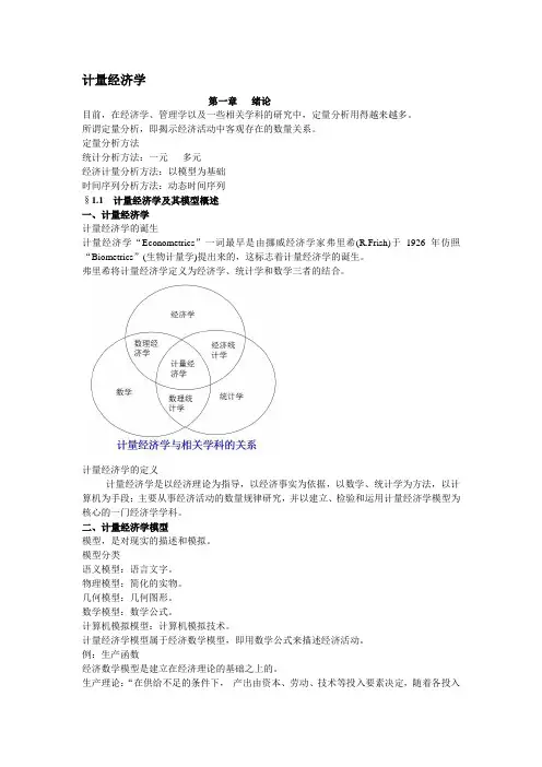
定量分析方法统计分析方法:一元多元经济计量分析方法:以模型为基础时间序列分析方法:动态时间序列§1.1 计量经济学及其模型概述一、计量经济学计量经济学的诞生计量经济学“Econometrics”一词最早是由挪威经济学家弗里希(R.Frish)于1926年仿照“Biometrics”(生物计量学)提出来的,这标志着计量经济学的诞生。
弗里希将计量经济学定义为经济学、统计学和数学三者的结合。
计量经济学的定义计量经济学是以经济理论为指导,以经济事实为依据,以数学、统计学为方法,以计算机为手段;主要从事经济活动的数量规律研究,并以建立、检验和运用计量经济学模型为核心的一门经济学学科。
二、计量经济学模型模型,是对现实的描述和模拟。
模型分类语义模型:语言文字。
物理模型:简化的实物。
几何模型:几何图形。
数学模型:数学公式。
计算机模拟模型:计算机模拟技术。
计量经济学模型属于经济数学模型,即用数学公式来描述经济活动。
例:生产函数经济数学模型是建立在经济理论的基础之上的。
生产理论:“在供给不足的条件下,产出由资本、劳动、技术等投入要素决定,随着各投入要素的增加,产出也随之增加,但要素的边际产出递减。
” 建立初始模型初始模型的特点模型描述了经济变量之间的理论关系;通过模型可以分析经济活动中各因素之间的相互影响,从而为控制经济活动提供理论指导;认为这种关系是准确实现的;模型并没有揭示各因素之间的定量关系,因为参数未知。
模型的改进以1964-1984年我国工业生产活动的数据作为样本,估计得到:改进模型的特点1.用随机性的数学方程描述现实的经济活动与经济关系。
2.揭示了经济活动中各因素之间的定量关系。
3.可用于对研究对象进行深入的研究,如结构分析、生产预测等。
初始模型——数理经济学模型数理经济学模型:由确定性的数学方程所构 成,用以揭示经济活动中各因素间的理论关系。


第八章向量自回归模型第一节平稳的V AR过程第二节 非限制性向量自回归模型的估计第三节 V AR模型的应用第四节 协整与误差校正模型第一节平稳的V AR过程一、 V AR过程的基本概念1980年Sims首先提出向量自回归模型(vector autoregressive model)。
这种模型采用多方程联立的形式,它不以经济理论为基础。
在模型的每一个方程中,内生变量对模型的全部内生变量的滞后项进行回归,从而估计全部内生变量的动态关系。
1单变量时间序列的AR(p)模型很容易推广到多元情形,这就是V AR(p)模型,它的定义为11t t p t p t y v A y A y u −−=++++ , 0,1,2,,t =±±… (8.1)这里t 1(,,)t t K y y y ′=…是一个1K ×维的随机向量,i A 是固定的K K ×维的系数矩阵,1(,,)K v v v ′=…是一个1K ×维的截距向量。
t 1(,,)t t K u u u ′=…是一个1K ×维的白噪声新息过程,亦即,()0t E u =()t t u E u u ′=Σ且()0t sE u u ′=(当s t ≠时)、||0u Σ≠。
两个变量y 1t ,y 2t 滞后1期的V AR 模型2111111122112221112221t t t t tt t t y v a y a y u y v a y a y u −−−−=+++⎧⎨=+++⎩其中u 1 t , u 2 t ∼ IID (0, σ 2), Cov(u 1 t , u 2 t ) = 0。
写成矩阵形式为11t t t y v A y u −=++,1,2,t =… 于是一般的V AR(1)模型如下(t y 可能包含不止两个变量)11t t t y v A y u −=++,1,2,t =… (8.2)容易推得21101y v A y u =++211211012()y v A y u v A v A y u u =++=++++2110112()K I A v A y Au u =++++类似地,可得1111101t i 0()t t t i t K i y I A A v A y A u −−−==+++++∑ 0()jj j i t K t j i i (8.3)从(8.3)式可以得到111111t y I A A v A y A u +−−−==+++++∑类似于一维情形,如果矩阵1A 的行列式的特征值都在单位圆外,则矩阵序列1iA ,0,1,i =…是绝对可和的,所以无限和式10it i i A u ∞−=∑存在均方极限。
WEEK 10: MACROECONOMETRICS Introduction1.The concept of stationarity2.Spurious regressions3.Testing for unit roots4.Cointegration analysis1. S TATIONARITYConditions for t y to be a stationary time series process i. t E y constant t ii. t Var y constant tiii. ,t t k Cov y y constant t and all k≠0 Autoregressive time series1t t t y y- Notice no constant and t is a white noise error term.- AR(1) model – time series behaviour of t y is largely explained by its value in the previous period.- Necessary condition for stationarity 1 , if , 1 series is explosive and if 1 have a unit root.Example 1 – Stationary AR(1) ModelSTATA codeset obs 500 /*set number of observations*/gen time=_n /*create time trend*/gen y=0 if time==1 /* first observation set y=0*/gen e=rnormal(0, 1) /*create a random number*/replace y=(0.67*y[_n-1])+e if time~=1 /*AR(1) model =0.67*/ twoway (line y time) /*line plot*/Example 2 – Explosive AR(1) ModelSTATA codeset obs 500 /*set number of observations*/gen time=_n /*create time trend*/gen y=0 if time==1 /* first observation set y=0*/gen e=rnormal(0, 1) /*create a random number*/replace y=(1.16*y[_n-1])+e if time~=1 /*AR(1) model =1.16*/ twoway (line y time) /*line plot*/Example 3 – Non-stationary AR(1) ModelSTATA codeset obs 500 /*set number of observations*/gen time=_n /*create time trend*/gen y=0 if time==1 /* first observation set y=0*/ gen e=rnormal(0, 1) /*create a random number*/ replace y=y[_n-1]+e if time~=1 /*AR(1) model =1*/ twoway (line x time) /*line plot*/ Noticety is not mean reverting. Random walk =1In the model:1t t t y yif 1 then t y is said to contain a UNIT ROOT i.e. is non-stationarySo 1t t t y y subtract 1t y from the LHS and RHS:111t t t t t y y y yt t y and because t is white noise t y is a stationary series.Example 3 (continued) – Non-stationary AR(1) Model and First Difference- A series t y is integrated of order one, i.e. t y I (1), and contains a unit root if t y is non-stationary but t y is a stationary series.- Possible that the series t y needs to be differenced more than once to achieve a stationary process.- A series t y is integrated of order d , i.e. t y I (d) if t y is non-stationary but d t y is a stationary series: Note: 211t t t t t t t y y y y y y y2.S PURIOUS REGRESSIONWhy worry whether t y is stationary?Most macroeconomic time series are trended and in most cases non-stationary processes.Using OLS to model non-stationary data can lead to problems and incorrect conclusions.a.high R squared often >0.95b.high t valuesc.theoretically variables in the analysis have no interrelationship Why does non-stationarity arise in macro data?Economic time series e.g. GDP, money supply, employment, all tend to grow at an annual rate.Such series non-stationary as the mean is continually rising. Even after differencing the series cannot be made stationary.So, usually take logarithms of time series data before undertaking econometric analysis.Take logarithm of a series which exhibits an average growth rate it will follow a linear trend and become an integrated series, i.e. one which is stationarity after differencing.Consider t y which grows by 10% per period, thus11.1t t y yTake the log of both the LHS and RHS, then1log log 1.1log t t y yThe lagged dependent variable has a unit coefficient and log 1.1 is a constant. The series would now be I(1), see example 3.Consider the model01t t t y xCLRM assumptions require that both variables have zero mean and constant variance (i.e. stationary, see (1i and 1ii)).If these assumption are violated and the series are non-stationary Granger and Newbold (1974) proved that results obtained are totally spurious. Granger, C. and P. Newbold (1974) Spurious regressions in econometrics. Journal of Econometrics, 2, 111-120.‘Rule of thumb’ for detecting a spurious regression:or,a.2R DWRb.12Logic behind spurious regression.Consider two unrelated series that are non-stationary, then:– both either together, or one will whilst the other .– Either way likely to find a +ve or –ve significant relationship.PROFESSOR KARL TAYLOR ECN6540 2017-18 Example 4 – Spurious Regression: Artificial DataSource | SS df MS Number of obs = 500-------------+------------------------------ F( 1, 498) = 143.04Model | 9096.19185 1 9096.19185 Prob > F = 0.0000Residual | 31668.4706 498 63.5913065 R-squared = 0.2231-------------+------------------------------ Adj R-squared = 0.2216Total | 40764.6625 499 81.6927104 Root MSE = 7.9744------------------------------------------------------------------------------y | Coef. Std. Err. t P>|t| [95% Conf. Interval]-------------+----------------------------------------------------------------x | .9443085 .0789556 11.96 0.000 .7891813 1.099436_cons | 3.505432 .4156699 8.43 0.000 2.688749 4.322114------------------------------------------------------------------------------ Durbin-Watson d-statistic (2, 500) = 0.0316917Example 5 – Spurious Regression: Economic DataRegress by OLS the logarithm of GDP against the logarithm of M2. Quarterly time series data over the period 1975Q1 until 1997Q4.01log log tt t gdp muse "C:\Karl's files\2016-17\ECN6540\LECTURES\spurious1.dta", cleargen date=q(1975q1)+_n-1format date %tq tsset dategen lgdp=log(gdp) gen lm=log(m) reg lgdp lm estat dwatsonSource | SS df MS Number of obs = 92 -------------+------------------------------ F( 1, 90) = 547.56 Model | 1.78659606 1 1.78659606 Prob > F = 0.0000 Residual | .29365627 90 .003262847 R-squared = 0.8588 -------------+------------------------------ Adj R-squared = 0.8573 Total | 2.08025233 91 .022859916 Root MSE = .05712 ------------------------------------------------------------------------------ lgdp | Coef. Std. Err. t P>|t| [95% Conf. Interval] -------------+---------------------------------------------------------------- lm | .219892 .0093971 23.40 0.000 .201223 .2385611 _cons | 3.075618 .0571457 53.82 0.000 2.962088 3.189147 ------------------------------------------------------------------------------ Durbin-Watson d-statistic( 2, 92) = 0.032836Regression fits the data well – both variables trended.Why is this regression spurious?In the model 01t t t y x there are four possible scenarios:a. Both t y and t x are stationary processes and so the CLRM is appropriate and OLS is BLUE;b. t y and t x are integrated of difference orders, e.g. I(0) and I(1), – the regression is now meaningless, since t y has a constant mean and t x drifts over time;c. t y and t x are integrated of the same order, e.g. I(1), and t contains a stochastic trend, i.e. I(1). This is the case of a spurious regression. Could re-estimate the model in first differences.d. t y and t x are integrated of the same order,e.g. I(1), and t is a stationary process, i.e. I(0). In this special case t y and t x are said to be cointegrated .Hence testing for non-stationarity is extremely important.3. T ESTING FOR UNIT ROOTSTesting the order of integration is a test for the number of unit roots.i. Test t y to see if stationary. If stationary then t y I (0); if not stationary then t y I (d); d >0.ii. Take first differences of t y i.e. 1t t t y y y then test t y to see ifstationary. If stationary then t y I (1); if not stationary then t y I (d); d >0.iii. Take the second difference of t y i.e. 21t t t t y y y y then test 2t yto see if stationary. If stationary then t y I (2); if not stationary then t y I (d); d >0.Continue process until stationary.Dickey-Fuller Test for Unit RootsDickey and Fuller (1979) Distribution of the estimators for autoregressive time series with a unit root. Journal of the American Statistical Association , 74, 427-431.Dickey and Fuller (1981) Likelihood ratio statistics for autoregressive time series with a unit root. Econometrica , 49, 1057-1072.Test based on testing for the existence of a unit root.Start with an AR(1) model:1t t t y yTo test for a unit root 0:1H 1:1HCan re-write the above model by subtracting 1t y from both sides:111111t t t t t tt t t t y y y y y y y(1)1To test for a unit root the null and alternative hypotheses are 0:0H 1:0HDickey and Fuller proposed two alternative regression equations which can be used for testing the presence of a unit root:1t t t y y (2)Testing for a unit root based upon eq. (1) is only valid if the d.g.p has a zero mean and no trend. So eq. (2) includes a constant in the random walk process.1t t t y t y (3)Allows for a non zero mean and trend component in the series.The DF test for a unit root is based upon a conventional t test on from one of the three models.Critical values (based upon Mackinnon, 1991): MODEL 1% 5% 10% 1t t t y y 1t t t y y -3.43 -2.86 -2.57 1t t t y t y -3.96 -3.41 -3.13 Standard critical values -2.33 -1.65 -1.28If t statistic is greater than the critical value then the null hypothesis of a unit root is rejected and can conclude that t y is a stationary process.3.1 Augmented Dickey-Fuller Test for Unit RootsUnlikely that the error term t in eqs. (1) to (3) is white noise – auto/serial correlation.Dickey and Fuller proposed augmenting the DF test by including extra lagged terms of the dependent variable to eliminate the presence of autocorrelation.11p k t k k t t t y y y (4)11p k t k k t t t y y y (5)11p k t k k t t t y y y t (6)Again the difference between eqs. (4) to (6) concerns the inclusion of a constant and trend.An important consideration is the optimal lag length p.-If p is too small then the remaining autocorrelation will bias the test.-If p is too large then the power of the test will suffer.Ng and Perron (1995) suggest firstly, set an upper bound for p i.e. p . Then estimate the ADF test based on the p lag length.If the absolute value of the t-statistic for testing the significance of the last lagged difference is greater than 1.6 then set p=p and perform the unit root test. Otherwise, reduce the lag length by one and repeat the process.Rule of thumb (Schwert, 1989),0.25int12100Tp3.2 Kwiatkowski-Phillips-Schmidt-Shin (1992)Testing the null hypothesis of stationarity against the alternative of a unit root. How sure are we that economic time series have a unit root? Journal of Econometrics , 54, 159-178.KPSS test differs to the DF and ADF null hypothesis is stationarity. Model decomposed into trend, random walk (t r ) and a stationary error term:21,0u t tt t tt t IID u u r r r t yThe initial value of t r is fixed and serves the role of the intercept 0r . Thestationary null hypothesis is that 20u since tis stationary, hence under the null hypothesis t y is trend stationary.To undertake the test:i. Regress t y of on an intercept and time trend, i.e. t t y t ;ii. Save the OLS residuals from (i) ˆt t eand compute the partial sum process, i.e. 1t s t s S e ;iii. Test statistic is LM, given by:221ˆT tt KPSS S .2ˆis an estimate of the error variance RSS/T (may be corrected for autocorrelation);iv. Critical value at 5% level 0.145. If trend omitted from (i) then the criticalvalue at the 5% level is 0.463.Example 6 – Unit Root Tests – ADF test: Nelson & Plosser U.S. Data Nelson, C.R. and Plosser, C.I. (1982), Trends and Random Walks in Macroeconomic Time Series, Journal of Monetary Economics, 10, 139–162.clear all /*clear memory*/use /ec-p/data/macro/nelsonplosser.dta /*load data*/ keep year lip lsp500 /*keep a subset of Nelson and Plosser variables*/drop if lip==. | lsp500==. /*drop any missing observation*/tsset year /*set year as time identifier*/twoway (line lip year) (line lsp500 year, yaxis(2)) /*plot data over time*//*ADF tests on industrial production*/dfuller lip, regress noconstant lags(3) /*ADF test no constant or trend eq.(4) */ dfuller lip, regress lags(3) /*ADF test constant no trend eq.(5) */dfuller lip, regress trend lags(3) /*ADF test constant and trend eq.(6) *//*ADF tests on S&P 500 index*/dfuller lsp500, regress noconstant lags(3) /*ADF test no constant or trend eq.(4) */ dfuller lsp500, regress lags(3) /*ADF test constant no trend eq.(5) */dfuller lsp500, regress trend lags(3) /*ADF test constant and trend eq.(6) *//*ADF tests on industrial production*/dfuller lip, regress noconstant lags(3) /*ADF test no constant or trend eq.(4) */ Augmented Dickey-Fuller test for unit root Number of obs = 96---------- Interpolated Dickey-Fuller ---------Test 1% Critical 5% Critical 10% CriticalStatistic Value Value Value------------------------------------------------------------------------------Z(t) 2.640 -2.602 -1.950 -1.610------------------------------------------------------------------------------D.lip | Coef. Std. Err. t P>|t| [95% Conf. Interval]-------------+----------------------------------------------------------------lip |L1. | .0121854 .0046149 2.64 0.010 .0030198 .0213511LD. | .0855473 .1060297 0.81 0.422 -.1250368 .2961313L2D. | -.0727104 .1059196 -0.69 0.494 -.2830758 .1376551L3D. | .0177574 .1045445 0.17 0.865 -.189877 .2253918------------------------------------------------------------------------------dfuller lip, regress lags(3) /*ADF test constant no trend eq.(5) */Augmented Dickey-Fuller test for unit root Number of obs = 96 ---------- Interpolated Dickey-Fuller --------- Test 1% Critical 5% Critical 10% Critical Statistic Value Value Value ------------------------------------------------------------------------------ Z(t) -0.687 -3.516 -2.893 -2.582 ------------------------------------------------------------------------------------------------------------------------------------------------------------ D.lip | Coef. Std. Err. t P>|t| [95% Conf. Interval] -------------+---------------------------------------------------------------- lip |L1. | -.006546 .0095294 -0.69 0.494 -.025475 .0123831 LD. | .05638 .1046247 0.54 0.591 -.1514442 .2642041 L2D. | -.0932085 .1041037 -0.90 0.373 -.2999977 .1135807 L3D. | -.0161771 .1034743 -0.16 0.876 -.2217161 .1893618 _cons | .0627725 .0281174 2.23 0.028 .0069208 .1186242 ------------------------------------------------------------------------------dfuller lip, regress trend lags(3) /*ADF test constant and trend eq.(6) */Augmented Dickey-Fuller test for unit root Number of obs = 96---------- Interpolated Dickey-Fuller --------- Test 1% Critical 5% Critical 10% Critical Statistic Value Value Value ------------------------------------------------------------------------------ Z(t) -3.298 -4.049 -3.454 -3.152 ------------------------------------------------------------------------------------------------------------------------------------------------------------ D.lip | Coef. Std. Err. t P>|t| [95% Conf. Interval] -------------+---------------------------------------------------------------- lip |L1. | -.2207902 .0669447 -3.30 0.001 -.3537874 -.0877929 LD. | .168619 .1054778 1.60 0.113 -.040931 .378169 L2D. | .0151678 .10462 0.14 0.885 -.1926782 .2230138 L3D. | .0831198 .1031807 0.81 0.423 -.1218666 .2881062 _trend | .0088867 .0027512 3.23 0.002 .0034209 .0143524 _cons | .1611592 .0405474 3.97 0.000 .0806046 .2417137 ------------------------------------------------------------------------------Note can find given 10.220810.220810.7792/*ADF tests on S&P 500 index*/dfuller lsp500, regress noconstant lags(3) /*ADF test no constant & trend eq.(4) */ Augmented Dickey-Fuller test for unit root Number of obs = 96---------- Interpolated Dickey-Fuller ---------Test 1% Critical 5% Critical 10% CriticalStatistic Value Value Value------------------------------------------------------------------------------Z(t) 1.567 -2.602 -1.950 -1.610------------------------------------------------------------------------------D.lsp500 | Coef. Std. Err. t P>|t| [95% Conf. Interval]-------------+----------------------------------------------------------------lsp500 |L1. | .0106279 .0067804 1.57 0.120 -.0028386 .0240944LD. | .2531512 .1064478 2.38 0.019 .0417367 .4645658L2D. | -.1932357 .107425 -1.80 0.075 -.406591 .0201196L3D. | -.017031 .1064838 -0.16 0.873 -.228517 .194455------------------------------------------------------------------------------dfuller lsp500, regress lags(3) /*ADF test constant no trend eq.(5) */ Augmented Dickey-Fuller test for unit root Number of obs = 96 ---------- Interpolated Dickey-Fuller --------- Test 1% Critical 5% Critical 10% Critical Statistic Value Value Value ------------------------------------------------------------------------------ Z(t) 0.059 -3.516 -2.893 -2.582 ------------------------------------------------------------------------------------------------------------------------------------------------------------ D.lsp500 | Coef. Std. Err. t P>|t| [95% Conf. Interval] -------------+---------------------------------------------------------------- lsp500 |L1. | .0011734 .0200279 0.06 0.953 -.0386096 .0409564 LD. | .2612615 .1080976 2.42 0.018 .046539 .475984 L2D. | -.1856923 .1089062 -1.71 0.092 -.4020212 .0306366 L3D. | -.0079754 .1084307 -0.07 0.942 -.2233596 .2074089 _cons | .0252099 .0502234 0.50 0.617 -.0745527 .1249725 ------------------------------------------------------------------------------dfuller lsp500, regress trend lags(3) /*ADF test constant and trend eq.(6) */ Augmented Dickey-Fuller test for unit root Number of obs = 96---------- Interpolated Dickey-Fuller ---------Test 1% Critical 5% Critical 10% CriticalStatistic Value Value Value------------------------------------------------------------------------------Z(t) -2.121 -4.049 -3.454 -3.152------------------------------------------------------------------------------------------------------------------------------------------------------------D.lsp500 | Coef. Std. Err. t P>|t| [95% Conf. Interval]-------------+----------------------------------------------------------------lsp500 |L1. | -.0969978 .0457218 -2.12 0.037 -.1878321 -.0061635LD. | .3015991 .1068021 2.82 0.006 .0894181 .5137802L2D. | -.1405117 .1079217 -1.30 0.196 -.3549171 .0738936L3D. | .0396776 .1076543 0.37 0.713 -.1741965 .2535517_trend | .0032803 .0013813 2.37 0.020 .0005362 .0060245_cons | .0942689 .0569704 1.65 0.101 -.0189127 .2074505------------------------------------------------------------------------------So both industrial production and the S&P 500 index definitely not stationary over the period, i.e. not I(0).Order of integration?Take first difference then undertake test again.In STATA the first difference operator is D, second difference operator is D2 /*ADF tests on industrial production first differenced*/dfuller D.lip, lags(3) /*ADF test constant no trend eq.(5) */dfuller D.lip, trend lags(3) /*ADF test constant and trend eq.(6) *//*ADF tests on S&P 500 index first differenced*/dfuller D.lsp500, lags(3) /*ADF test constant no trend eq.(5) */dfuller D.lsp500, trend lags(3) /*ADF test constant and trend eq.(6) *//*ADF tests on industrial production first differenced*/dfuller D.lip, lags(3) /*ADF test constant no trend eq.(5) */Augmented Dickey-Fuller test for unit root Number of obs = 95 ---------- Interpolated Dickey-Fuller --------- Test 1% Critical 5% Critical 10% Critical Statistic Value Value Value ------------------------------------------------------------------------------ Z(t) -5.624 -3.517 -2.894 -2.582 ------------------------------------------------------------------------------dfuller D.lip, trend lags(3) /*ADF test constant and trend eq.(6) */ Augmented Dickey-Fuller test for unit root Number of obs = 95---------- Interpolated Dickey-Fuller --------- Test 1% Critical 5% Critical 10% Critical Statistic Value Value Value ------------------------------------------------------------------------------ Z(t) -5.600 -4.051 -3.455 -3.153 ------------------------------------------------------------------------------/*ADF tests on S&P 500 index first differenced*/dfuller D.lsp500, lags(3) /*ADF test constant no trend eq.(5) */Augmented Dickey-Fuller test for unit root Number of obs = 95 ---------- Interpolated Dickey-Fuller --------- Test 1% Critical 5% Critical 10% Critical Statistic Value Value Value ------------------------------------------------------------------------------ Z(t) -5.996 -3.517 -2.894 -2.582 ------------------------------------------------------------------------------dfuller D.lsp500, trend lags(3) /*ADF test constant and trend eq.(6) */ Augmented Dickey-Fuller test for unit root Number of obs = 95---------- Interpolated Dickey-Fuller --------- Test 1% Critical 5% Critical 10% Critical Statistic Value Value Value ------------------------------------------------------------------------------ Z(t) -6.149 -4.051 -3.455 -3.153 ------------------------------------------------------------------------------Hence both industrial production and the S&P 500 index are I(1).4.C OINTEGRATION-Trended data can create problems due to spurious regressions.-Most macro variables are trended and hence non-stationary.-Hence the problem of spurious regressions is likely in macro models. Solution?Difference the data until it becomes stationary.Problemsi.If the model is correctly specified in both y and x then differencing bothvariables means the error process is also differenced non-invertibleMA process, estimation difficulties;ii.Once the model is differenced it can no longer have a unique long run solution.4.1 Cointegration DefinitionsWhere the regression of one non-stationary variable y on one or more non-stationary variables ,,,12k x x x results in a non spurious regression.Then a long run equilibrium relationship exists between the variables.Hence cointegration should only occur where there is a relationship linking the variables.We will only consider the case of two variables t y and t x i.e. not multivariate cointegration.If there is a long run equilibrium relationship between t y and t x , despite them both rising over time (trended), then a linear combination of the two variables must be I(0).A linear combination can be taken from the model:01t t t y xConsider the residuals:01ˆˆˆt t t t e y xIf t e I (0) then t y and t x are said to be cointegrated.10, is known as the cointegrating vector.Definitions:i. Time series t y and t x cointegrated of order d , b where d ≥b ≥0, which canbe written as t t x y , CI (d,b ), if both series are I(d ) and a linear combinationexists between the variables integrated of order I(d-b ). Then ,12 is the cointegrating vector (there is only one).ii. Generalisation, multivariate cointegration: let t Z denote an n×1 vector ofthe series ,,,,123nt t t t Z Z Z Z , if each it Z is I(d ) and an n×1 vector exists such that ' t Z I (d-b ) then it Z CI (d,b ). Can be more than one cointegrating vector.4.2Testing for Cointegration in single equationsEngle, R. and C. Granger (1987) Cointegration and error correction: Representation, estimation and testing. Econometrica, 35, 251-276.Step 1-By definition cointegration requires that the variables are integrated of the same order I(d).-So apply ADF tests to infer the number of unit roots in each variable.i.If both t y and t x are I(0) then OLS and appropriate.ii.If t y and t x are integrated to different orders, e.g. I(0) and I(1), then they can-not be cointegrated.iii.If both t y and t x are integrated to the same order, e.g. I(1), then go to step 2.Step 2- If both t y and t x are integrated to the same order, in macro data usually I(1), then estimate the long run equilibrium relationship:01t t t y x- Obtain the residuals from the model, t e .- If there is no cointegration then the results will be spurious (see section 2).- If the variables are cointegrated then OLS yields super-consistent estimatesfor the cointegrating parameter 1ˆ .Step 3- Test the residuals from step 2 for stationarity using the ADF test:11p k t k k t t t u e e e- If t e I (0) then t y and t x are cointegrated.- Note critical value differ to those standard ADF tests:Critical values (based upon Engle-Granger, 1987): MODEL 1% 5% 10%Lags (ADF) -3.73 -3.17-2.91Example 7 – Engle Granger Cointegration Use King et al. data for the U.S.:King, R. G., C. I. Plosser, J. H. Stock, and M. W. Watson. 1991. Stochastic trends and economic fluctuations. American Economic Review , 81, 819–840.Model logarithm of consumption (c) as a function of the logarithm of gdp (y).01log log t t t c yclear all /*clear memory*/use /data/r11/balance2 /*load data*/ tsset time /*set year as time identifier*/ twoway (line y time) (line c time, yaxis(2))/*STEP 1 - order of integration*//*ADF tests on real gdp*/dfuller y, regress trend lags(4) /*ADF test constant and trend eq.(6)*/ /*ADF tests on consumption*/dfuller c, regress trend lags(4) /*ADF test constant and trend eq.(6)*/ /*STEP 2 - estimate long run relationship*/regress c ypredict e, resid /*gain residuals*/estat dwatson /*durbin watson statistic*//*STEP 3 - test residuals for stationarity*/dfuller e, regress noconstant lags(4) /*ADF test on residual*//*step 1 - order of integration*//*ADF tests on real gdp*/Dfuller y, regress trend lags(4) /*ADF test constant and trend eq.(6)*/Augmented Dickey-Fuller test for unit root Number of obs = 91---------- Interpolated Dickey-Fuller --------- Test 1% Critical 5% Critical 10% Critical Statistic Value Value Value ------------------------------------------------------------------------------ Z(t) -2.133 -4.060 -3.459 -3.155 ------------------------------------------------------------------------------------------------------------------------------------------------------------ D.y | Coef. Std. Err. t P>|t| [95% Conf. Interval] -------------+---------------------------------------------------------------- y |L1. | -.0089805 .0042109 -2.13 0.036 -.0173543 -.0006067 LD. | .6394239 .1096428 5.83 0.000 .4213873 .8574606 L2D. | -.0055359 .1296175 -0.04 0.966 -.2632945 .2522227 L3D. | .0906288 .1302257 0.70 0.488 -.1683393 .3495969 L4D. | .0008952 .1130575 0.01 0.994 -.2239321 .2257225 _trend | .0001668 .0000632 2.64 0.010 .0000411 .0002926 _cons | .0260383 .0118528 2.20 0.031 .0024678 .0496088 ------------------------------------------------------------------------------/*ADF tests on consumption*/dfuller c, regress trend lags(4) /*ADF test constant and trend eq.(6)*/ Augmented Dickey-Fuller test for unit root Number of obs = 91 ---------- Interpolated Dickey-Fuller --------- Test 1% Critical 5% Critical 10% Critical Statistic Value Value Value ------------------------------------------------------------------------------ Z(t) -1.622 -4.060 -3.459 -3.155 ------------------------------------------------------------------------------------------------------------------------------------------------------------ D.c | Coef. Std. Err. t P>|t| [95% Conf. Interval] -------------+---------------------------------------------------------------- c |L1. | -.0063104 .0038897 -1.62 0.108 -.0140456 .0014248 LD. | .6579478 .1068026 6.16 0.000 .4455591 .8703365 L2D. | .1038069 .1289307 0.81 0.423 -.152586 .3601998 L3D. | .2031445 .1317853 1.54 0.127 -.0589249 .465214 L4D. | -.2282238 .1125153 -2.03 0.046 -.4519729 -.0044747 _trend | .0001326 .0000526 2.52 0.014 .0000279 .0002372 _cons | .0180606 .0109068 1.66 0.101 -.0036288 .0397499 ------------------------------------------------------------------------------。