数字信号处理 DSP 英文版课件4.0

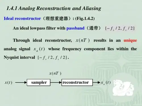
数字信号处理Digital Signal Processing 电子信息工程系韩建峰KeywordsSections⏹Sampling sinusoids⏹Sampling theorem⏹Discrete-to-Continuous Conversion SummaryLECTURE 1Reading assignments This lecture •Chapter 4•Section 4-1KeywordsPart AContinuous-to-Discrete Conversion Sampling & ReconstructionAliasing & FoldingLECTURE OBJECTIVES•SAMPLING can cause ALIASING •Spectrum for digital signals,x [n]•Normalized Frequencyππωω22ˆ+==ss f f T ALIASINGReviewSignalsSampling Reconstruction•Continuous-time Signal•But the key point is that any computer represent ation is discrete.•So, do sampling!•And, how?()cos()x t A tωϕ=+•Sample a continuous-time signal at equally spaced time instants.Take a “snapshot” every Ts.Speech, audio andso on.•Or, compute the values of a discrete-time signal directly from a formula.2=-+[]53x n n nSAMPLING x(t)•SAMPLING PROCESS•Convert x(t) to numbers x[n]•“n” is an integer; x[n] is a sequence ofvalues•Think of “n” as the storage address inmemory•UNIFORM SAMPLING at t = nTs•IDEAL: x[n] = x(nT)sSAMPLING RATE, f s •SAMPLING RATE (f)s–f=1/T ss•NUMBER of SAMPLES PER SECOND –T= 125 microsec f s= 8000 samples/secs–UNITS ARE HERTZ: 8000 Hz •UNIFORM SAMPLING at t = nT= n/f ss–IDEAL: x[n] = x(nT)=x(n/f s)s•Examples of continuous-time signals exist in the “real-world” outside the computer.•Simple mathematical formula.•More general continuous-time signals can be represented as sum of sinusoids.•So, we will use sinusoidal signal as the basis for our study of sampling.sf s T n A n x ωωωϕω==+=ˆ)ˆcos(][)cos()(][)cos()(ϕωϕω+==+=s s nT A nT x n x t A t x •Change x(t) into x[n] DERIV ATION))cos((][ϕω+=n T A n x s DEFINE DIGITAL FREQUENCYDigital Frequency ωˆ•V ARIES from 0to 2π, as f varies from 0 to the sampling frequency•UNITS are radians, not rad/sec–DIGITAL FREQUENCY is NORMALIZEDss f f T πωω2ˆ==Sample RateHow to select theT sSample TheoremA interesting phenomenon•Exercise 4.1•Is this the only possible answer?Hz 1000at sampled )2400cos()(2==s f t t x π21000[]cos(2400)cos(2.4)cos(0.42)cos(0.4)nx n n n n n πππππ===+=()cos(400)x t t π⇒=Aliasing[]cos(0.4)x n n π=Illustration of aliasingDifferent frequency, but same values at n=0,1,2,3…•2.4πis an alias of 0.4π•Exercise 4.2Aliasing•How does aliasing arise in a mathematical treat ment of discrete-time signal?•The last example:12[]cos(0.4)[]cos(2.4)x n n x n n ππ==2[]cos(0.42)cos(0.4)x n n n n πππ=+=Periodic function with period 2πAliasing Derivation-1and we substitute: t ←n f sIf x (t )=A cos(2π(f + f s )t +ϕ)then: x [n ]=A cos(2π(f + f s )n f s +ϕ)or, x [n ]=A cos(2πf f s n +2π n +ϕ)Aliasing Derivation-22ˆs sfT f πωω==+2π 2()22ˆthen: s s s s sf f f f f f f πππω+==+ˆand we want: []cos()x n A n ωϕ=+If x (t )=A cos(2π(f + f s )t +ϕ)t ←nf sFolded Aliasx (t )=A cos(2π(-f + f s )t -ϕ)SAME DIGITAL SIGNALˆ[]cos()x n A n ωϕ=+x [n ]=A cos((2πf T s )n -2π n +ϕ) x [n ]=A cos((-2πfT s )n +(2π f s T s )n -ϕ)x [n ]=x (nT s )=A cos(2π(-f + f s )nT s -ϕ)Aliasing2ˆs sfT f πωω==+2π 2ˆ2s sfT f πωωπ==-+Folded AliasAlisingPrincipal Aliasingˆˆˆ, 2, 2 integer l l l ωωππω+-=General FormulaSpectrum of a Discrete-Time Signal•PLOT versus NORMALIZED FREQUENCY •INCLUDE ALL SPECTRUM LINES –ALIASES•ADD MULTIPLES of 2π•SUBTRACT MULTIPLES of 2π–FOLDED ALIASES•ALIASES of NEGATIVE FREQS12X*–0.5π12X–1.5π12X0.5π2.5π–2.5πˆω12X12X*12X*1.5π))80/)(100(2cos(][ϕπ+=n A n x 80s f Hz=sf fπω2ˆ=ˆ2sff ωπ=f s =125Hz12X*0.4π12X–0.4π1.6π–1.6πˆω12X12X*))125/)(100(2cos(][ϕπ+=n A n x•DEMO: Strobe Movies 12•What is the meaning of this DEMO?•Can you give us more examples in the real world?f Camera: 30 Frames/s Human Eyessf'fSummary2ˆs sfT f πωω==+2π 2ˆ2s sfT f πωωπ==-+Folded AliasAlisingPrincipal Aliasingˆˆˆ, 2, 2 integer l l l ωωππω+-=General FormulaHomeworkP-4.1Review: Chapter 4, Section 4-1 Preview:Chapter 4, Section 4-2,4-4。

Digital Signal Processing Using Computer-Based Methods -Course Design for the 4th EditionIntroductionDigital Signal Processing (DSP) is an area of study that has witnessed significant growth and advancement in recent times. Technological advancements have made it possible to work with signals and signals processing methods more effectively and efficiently. The use of computers has also contributed significantly to the development of DSP methods. In this course design, we will provide an overview of the Digital Signal Processing course designed for the 4th edition of the book titled Digital Signal Processing Using Computer-Based Methods.Overview of the CourseThis course is designed to provide students with a fundamental understanding of digital signal processing concepts, their applications, and techniques for analyzing signals. The course is divided into eight modules, covering the following topics:1.Introduction to Digital Signal Processing2.Discrete-Time Signals and Systems3.Discrete Fourier Transform4.Z-Transform and Analysis of LTI Systems5.FIR Filter Design6.IIR Filter Design7.Multirate Signal Processing8.DSP Applications in Speech and Image ProcessingThe course will cover both theoretical and practical aspects of DSP, including hands-on experience with MATLAB software. The course involves lectures, discussions, and assignments, which will enable students to develop an in-depth understanding of DSP concepts and their applications.Course ObjectivesThe primary objectives of this course are to: - Develop an in-depth understanding of digital signal processing concepts and techniques - Familiarize students with the use of MATLAB for signal analysis and processing - Develop skills for designing digital filters and analyzing signals using the Fourier and Z-transforms - Provide practical experience with signal processing applications in speech and image processingCourse OutlineModule 1: Introduction to Digital Signal Processing •Basic concepts of digital signal processing•Analog-to-digital conversion•Sampling theorem•Signal quantizationModule 2: Discrete-Time Signals and Systems•Discrete-time signals and their characteristics•Discrete-time systems and their properties•Convolution and correlation of discrete-time signalsModule 3: Discrete Fourier Transform•Fourier series and Fourier Transform•Discrete Fourier Transform (DFT) and its properties •Fast Fourier Transform (FFT) algorithmsModule 4: Z-Transform and Analysis of LTI Systems •Z-Transform and its properties•Transfer function and Frequency Response of LTI systems•Analysis of LTI systems using Z-TransformModule 5: FIR Filter Design•Design of Finite Impulse Response (FIR) filters•Windowing techniques and their effects•Filter design using Fourier SeriesModule 6: IIR Filter Design•Design of Infinite Impulse Response (IIR) filters•Pole-zero locations and their effects•Butterworth and Chebyshev filter designs Module 7: Multirate Signal Processing•Sampling rate conversion using decimation and interpolation•Polyphase decomposition and filter banks•Multistage decimation and interpolation Module 8: DSP Applications in Speech and Image Processing •Speech analysis and synthesis•Speech coding and compression•Image enhancement and restoration•Image compressionEvaluationThe grading for this course will be based on your performance in the following components: - Regularassignments and quizzes: 20% - Mid-term examination: 30% - Final examination: 50%ConclusionThis course in Digital Signal Processing will provide students with a comprehensive understanding of digital signal processing concepts and their applications. The course will focus on fundamental principles, practical applications, and hands-on experience with digital signal processing using MATLAB. Upon successful completion of this course, students will have the skills and knowledge to analyze and design digital signal processing systems.。