伍德里奇《计量经济学导论--现代观点》

计量经济学应用研究的可信性革命在过去的几十年中，计量经济学作为经济学的一个重要分支，已经经历了两次可信性革命。

这些革命彻底改变了我们对于计量经济学应用研究可信性的理解和实践。

第一次可信性革命发生在20世纪70年代，以弗朗哥·魁奈尔（Franco Modigliani）和默顿·米勒（Merton Miller）的诺贝尔经济学奖获奖研究——MM定理（Modigliani-Miller Theorem）为标志。

MM定理为企业的投资决策和财务政策提供了新的视角，并改变了经济学家对于公司财务政策的研究方向。

这一理论革命强调了如果一个公司的投资决策和财务政策不受到税收、破产成本、以及代理关系等因素的影响，那么公司的投资决策和财务政策将与企业的市场价值无关。

这一革命性的研究为后来的企业金融、资产定价和宏观经济学等领域的研究提供了重要的理论基础。

第二次可信性革命发生在21世纪初，以本·伯南克（Ben Bernanke）和亚当·斯密（Adam Smith）的宏观经济理论为标志。

他们强调了货币政策对于稳定经济的重要性，并提出了一个基于“流动性陷阱”和“自然失业率”的理论框架来解释经济周期。

这一理论框架强调了中央银行通过控制货币供应量来稳定经济的必要性，以及经济中的结构性因素如劳动力市场和金融市场的不完善对于宏观经济稳定的影响。

这一革命性的研究为后来的货币政策制定、经济周期分析以及国际经济政策协调等领域的研究提供了重要的理论基础。

今天，我们正处在一个新的可信性革命的边缘。

以大数据和人工智能为代表的新兴技术正在对计量经济学应用研究产生深远的影响。

大数据的出现使得我们能够处理和分析了更多的数据，而人工智能则帮助我们更加深入地挖掘和理解这些数据背后的经济规律和趋势。

大数据已经改变了计量经济学应用研究的范式。

传统的计量经济学研究通常依赖于假设和简化现实世界的复杂性。

然而，大数据为我们提供了一个更为接近现实的、复杂的数据世界，使我们能够更准确地刻画和理解经济现象。

《计量经济学导论》考研伍德里奇考研复习笔记二第1章计量经济学的性质与经济数据1.1 复习笔记一、什么是计量经济学计量经济学是以一定的经济理论为基础，运用数学与统计学的方法，通过建立计量经济模型，定量分析经济变量之间的关系。

在进行计量分析时，首先需要利用经济数据估计出模型中的未知参数，然后对模型进行检验，在模型通过检验后还可以利用计量模型来进行预测。

在进行计量分析时获得的数据有两种形式，实验数据与非实验数据：（1）非实验数据是指并非从对个人、企业或经济系统中的某些部分的控制实验而得来的数据。

非实验数据有时被称为观测数据或回顾数据，以强调研究者只是被动的数据搜集者这一事实。

（2）实验数据通常是通过实验所获得的数据，但社会实验要么行不通要么实验代价高昂，所以在社会科学中要得到这些实验数据则困难得多。

二、经验经济分析的步骤经验分析就是利用数据来检验某个理论或估计某种关系。

1．对所关心问题的详细阐述问题可能涉及到对一个经济理论某特定方面的检验，或者对政府政策效果的检验。

2构造经济模型经济模型是描述各种经济关系的数理方程。

3经济模型变成计量模型先了解一下计量模型和经济模型有何关系。

与经济分析不同，在进行计量经济分析之前，必须明确函数的形式，并且计量经济模型通常都带有不确定的误差项。

通过设定一个特定的计量经济模型，我们就知道经济变量之间具体的数学关系，这样就解决了经济模型中内在的不确定性。

在多数情况下，计量经济分析是从对一个计量经济模型的设定开始的，而没有考虑模型构造的细节。

一旦设定了一个计量模型，所关心的各种假设便可用未知参数来表述。

4搜集相关变量的数据5用计量方法来估计计量模型中的参数，并规范地检验所关心的假设在某些情况下，计量模型还用于对理论的检验或对政策影响的研究。

三、经济数据的结构1横截面数据（1）横截面数据集，是指在给定时点对个人、家庭、企业、城市、州、国家或一系列其他单位采集的样本所构成的数据集。

伍德里奇计量经济学笔记伍德里奇计量经济学（Wooldridge Econometrics）是一门应用计量经济学的学科，它结合了经济学和数理统计学的理论和方法。

1. 引言- 计量经济学的定义：利用数理统计学和计量经济模型来分析经济问题。

- 经济学模型包括描述经济系统和理论关系的方程。

- 计量经济学的目标是估计和测试经济模型中的参数。

2. 统计学基础- 假设检验：用统计方法来验证经济理论。

- 最小二乘法（OLS）：估计经济模型中未知参数的方法。

- OLS估计结果的性质和假设：无偏性、一致性和有效性。

3. 单变量回归模型- 简单线性回归模型：一个自变量和一个因变量之间的线性关系。

- 估计参数和评估模型：OLS估计、t统计量、R方和调整的R 方。

- 解释和预测：利用估计的模型进行解释和预测。

4. 多变量回归模型- 多元线性回归模型：多个自变量和一个因变量之间的线性关系。

- 估计参数和评估模型：OLS估计、t统计量、F统计量、R方和调整的R方。

- 控制变量和决策：利用控制变量来减少混淆因素，做出更准确的决策。

5. 动态模型- 差分方程：描述变量随时间变化的关系。

- 滞后变量和滞后因变量：引入滞后变量来解释变量之间的时序关系。

- 动态因果关系：解释一些经济变量之间的长期和短期关系。

6. 面板数据模型- 面板数据：包含多个个体和多个时间观测的数据集。

- 固定效应模型和随机效应模型：解释面板数据中个体效应和时间效应。

- 引入个体和时间固定效应：控制个体特征和时间变化对变量关系的影响。

7. 工具变量估计- 决定性和随机性端变量：用于解决内生性问题的变量。

- 工具变量的选择和检验：选择有效的工具变量来估计内生性模型。

- 两阶段最小二乘法（2SLS）：用工具变量估计内生性模型。

8. 非线性回归模型- 非线性函数：描述实际经济关系的复杂性。

- 估计非线性模型：使用非线性最小二乘法（NLS）估计非线性模型。

- 非线性回归模型的解释和预测：利用估计的非线性模型进行解释和预测。

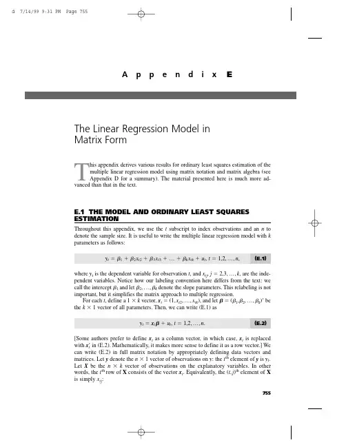
T his appendix derives various results for ordinary least squares estimation of themultiple linear regression model using matrix notation and matrix algebra (see Appendix D for a summary). The material presented here is much more ad-vanced than that in the text.E.1THE MODEL AND ORDINARY LEAST SQUARES ESTIMATIONThroughout this appendix,we use the t subscript to index observations and an n to denote the sample size. It is useful to write the multiple linear regression model with k parameters as follows:y t ϭ␤1ϩ␤2x t 2ϩ␤3x t 3ϩ… ϩ␤k x tk ϩu t ,t ϭ 1,2,…,n ,(E.1)where y t is the dependent variable for observation t ,and x tj ,j ϭ 2,3,…,k ,are the inde-pendent variables. Notice how our labeling convention here differs from the text:we call the intercept ␤1and let ␤2,…,␤k denote the slope parameters. This relabeling is not important,but it simplifies the matrix approach to multiple regression.For each t ,define a 1 ϫk vector,x t ϭ(1,x t 2,…,x tk ),and let ␤ϭ(␤1,␤2,…,␤k )Јbe the k ϫ1 vector of all parameters. Then,we can write (E.1) asy t ϭx t ␤ϩu t ,t ϭ 1,2,…,n .(E.2)[Some authors prefer to define x t as a column vector,in which case,x t is replaced with x t Јin (E.2). Mathematically,it makes more sense to define it as a row vector.] We can write (E.2) in full matrix notation by appropriately defining data vectors and matrices. Let y denote the n ϫ1 vector of observations on y :the t th element of y is y t .Let X be the n ϫk vector of observations on the explanatory variables. In other words,the t th row of X consists of the vector x t . Equivalently,the (t ,j )th element of X is simply x tj :755A p p e n d i x EThe Linear Regression Model inMatrix Formn X ϫ k ϵϭ .Finally,let u be the n ϫ 1 vector of unobservable disturbances. Then,we can write (E.2)for all n observations in matrix notation :y ϭX ␤ϩu .(E.3)Remember,because X is n ϫ k and ␤is k ϫ 1,X ␤is n ϫ 1.Estimation of ␤proceeds by minimizing the sum of squared residuals,as in Section3.2. Define the sum of squared residuals function for any possible k ϫ 1 parameter vec-tor b asSSR(b ) ϵ͚nt ϭ1(y t Ϫx t b )2.The k ϫ 1 vector of ordinary least squares estimates,␤ˆϭ(␤ˆ1,␤ˆ2,…,␤ˆk )؅,minimizes SSR(b ) over all possible k ϫ 1 vectors b . This is a problem in multivariable calculus.For ␤ˆto minimize the sum of squared residuals,it must solve the first order conditionѨSSR(␤ˆ)/Ѩb ϵ0.(E.4)Using the fact that the derivative of (y t Ϫx t b )2with respect to b is the 1ϫ k vector Ϫ2(y t Ϫx t b )x t ,(E.4) is equivalent to͚nt ϭ1xt Ј(y t Ϫx t ␤ˆ) ϵ0.(E.5)(We have divided by Ϫ2 and taken the transpose.) We can write this first order condi-tion as͚nt ϭ1(y t Ϫ␤ˆ1Ϫ␤ˆ2x t 2Ϫ… Ϫ␤ˆk x tk ) ϭ0͚nt ϭ1x t 2(y t Ϫ␤ˆ1Ϫ␤ˆ2x t 2Ϫ… Ϫ␤ˆk x tk ) ϭ0...͚nt ϭ1x tk (y t Ϫ␤ˆ1Ϫ␤ˆ2x t 2Ϫ… Ϫ␤ˆk x tk ) ϭ0,which,apart from the different labeling convention,is identical to the first order condi-tions in equation (3.13). We want to write these in matrix form to make them more use-ful. Using the formula for partitioned multiplication in Appendix D,we see that (E.5)is equivalent to΅1x 12x 13...x 1k1x 22x 23...x 2k...1x n 2x n 3...x nk ΄΅x 1x 2...x n ΄Appendix E The Linear Regression Model in Matrix Form756Appendix E The Linear Regression Model in Matrix FormXЈ(yϪX␤ˆ) ϭ0(E.6) or(XЈX)␤ˆϭXЈy.(E.7)It can be shown that (E.7) always has at least one solution. Multiple solutions do not help us,as we are looking for a unique set of OLS estimates given our data set. Assuming that the kϫ k symmetric matrix XЈX is nonsingular,we can premultiply both sides of (E.7) by (XЈX)Ϫ1to solve for the OLS estimator ␤ˆ:␤ˆϭ(XЈX)Ϫ1XЈy.(E.8)This is the critical formula for matrix analysis of the multiple linear regression model. The assumption that XЈX is invertible is equivalent to the assumption that rank(X) ϭk, which means that the columns of X must be linearly independent. This is the matrix ver-sion of MLR.4 in Chapter 3.Before we continue,(E.8) warrants a word of warning. It is tempting to simplify the formula for ␤ˆas follows:␤ˆϭ(XЈX)Ϫ1XЈyϭXϪ1(XЈ)Ϫ1XЈyϭXϪ1y.The flaw in this reasoning is that X is usually not a square matrix,and so it cannot be inverted. In other words,we cannot write (XЈX)Ϫ1ϭXϪ1(XЈ)Ϫ1unless nϭk,a case that virtually never arises in practice.The nϫ 1 vectors of OLS fitted values and residuals are given byyˆϭX␤ˆ,uˆϭyϪyˆϭyϪX␤ˆ.From (E.6) and the definition of uˆ,we can see that the first order condition for ␤ˆis the same asXЈuˆϭ0.(E.9) Because the first column of X consists entirely of ones,(E.9) implies that the OLS residuals always sum to zero when an intercept is included in the equation and that the sample covariance between each independent variable and the OLS residuals is zero. (We discussed both of these properties in Chapter 3.)The sum of squared residuals can be written asSSR ϭ͚n tϭ1uˆt2ϭuˆЈuˆϭ(yϪX␤ˆ)Ј(yϪX␤ˆ).(E.10)All of the algebraic properties from Chapter 3 can be derived using matrix algebra. For example,we can show that the total sum of squares is equal to the explained sum of squares plus the sum of squared residuals [see (3.27)]. The use of matrices does not pro-vide a simpler proof than summation notation,so we do not provide another derivation.757The matrix approach to multiple regression can be used as the basis for a geometri-cal interpretation of regression. This involves mathematical concepts that are even more advanced than those we covered in Appendix D. [See Goldberger (1991) or Greene (1997).]E.2FINITE SAMPLE PROPERTIES OF OLSDeriving the expected value and variance of the OLS estimator ␤ˆis facilitated by matrix algebra,but we must show some care in stating the assumptions.A S S U M P T I O N E.1(L I N E A R I N P A R A M E T E R S)The model can be written as in (E.3), where y is an observed nϫ 1 vector, X is an nϫ k observed matrix, and u is an nϫ 1 vector of unobserved errors or disturbances.A S S U M P T I O N E.2(Z E R O C O N D I T I O N A L M E A N)Conditional on the entire matrix X, each error ut has zero mean: E(ut͉X) ϭ0, tϭ1,2,…,n.In vector form,E(u͉X) ϭ0.(E.11) This assumption is implied by MLR.3 under the random sampling assumption,MLR.2.In time series applications,Assumption E.2 imposes strict exogeneity on the explana-tory variables,something discussed at length in Chapter 10. This rules out explanatory variables whose future values are correlated with ut; in particular,it eliminates laggeddependent variables. Under Assumption E.2,we can condition on the xtjwhen we com-pute the expected value of ␤ˆ.A S S U M P T I O N E.3(N O P E R F E C T C O L L I N E A R I T Y) The matrix X has rank k.This is a careful statement of the assumption that rules out linear dependencies among the explanatory variables. Under Assumption E.3,XЈX is nonsingular,and so ␤ˆis unique and can be written as in (E.8).T H E O R E M E.1(U N B I A S E D N E S S O F O L S)Under Assumptions E.1, E.2, and E.3, the OLS estimator ␤ˆis unbiased for ␤.P R O O F:Use Assumptions E.1 and E.3 and simple algebra to write␤ˆϭ(XЈX)Ϫ1XЈyϭ(XЈX)Ϫ1XЈ(X␤ϩu)ϭ(XЈX)Ϫ1(XЈX)␤ϩ(XЈX)Ϫ1XЈuϭ␤ϩ(XЈX)Ϫ1XЈu,(E.12)where we use the fact that (XЈX)Ϫ1(XЈX) ϭIk . Taking the expectation conditional on X givesAppendix E The Linear Regression Model in Matrix Form 758E(␤ˆ͉X)ϭ␤ϩ(XЈX)Ϫ1XЈE(u͉X)ϭ␤ϩ(XЈX)Ϫ1XЈ0ϭ␤,because E(u͉X) ϭ0under Assumption E.2. This argument clearly does not depend on the value of ␤, so we have shown that ␤ˆis unbiased.To obtain the simplest form of the variance-covariance matrix of ␤ˆ,we impose the assumptions of homoskedasticity and no serial correlation.A S S U M P T I O N E.4(H O M O S K E D A S T I C I T Y A N DN O S E R I A L C O R R E L A T I O N)(i) Var(ut͉X) ϭ␴2, t ϭ 1,2,…,n. (ii) Cov(u t,u s͉X) ϭ0, for all t s. In matrix form, we canwrite these two assumptions asVar(u͉X) ϭ␴2I n,(E.13)where Inis the nϫ n identity matrix.Part (i) of Assumption E.4 is the homoskedasticity assumption:the variance of utcan-not depend on any element of X,and the variance must be constant across observations, t. Part (ii) is the no serial correlation assumption:the errors cannot be correlated across observations. Under random sampling,and in any other cross-sectional sampling schemes with independent observations,part (ii) of Assumption E.4 automatically holds. For time series applications,part (ii) rules out correlation in the errors over time (both conditional on X and unconditionally).Because of (E.13),we often say that u has scalar variance-covariance matrix when Assumption E.4 holds. We can now derive the variance-covariance matrix of the OLS estimator.T H E O R E M E.2(V A R I A N C E-C O V A R I A N C EM A T R I X O F T H E O L S E S T I M A T O R)Under Assumptions E.1 through E.4,Var(␤ˆ͉X) ϭ␴2(XЈX)Ϫ1.(E.14)P R O O F:From the last formula in equation (E.12), we haveVar(␤ˆ͉X) ϭVar[(XЈX)Ϫ1XЈu͉X] ϭ(XЈX)Ϫ1XЈ[Var(u͉X)]X(XЈX)Ϫ1.Now, we use Assumption E.4 to getVar(␤ˆ͉X)ϭ(XЈX)Ϫ1XЈ(␴2I n)X(XЈX)Ϫ1ϭ␴2(XЈX)Ϫ1XЈX(XЈX)Ϫ1ϭ␴2(XЈX)Ϫ1.Appendix E The Linear Regression Model in Matrix Form759Formula (E.14) means that the variance of ␤ˆj (conditional on X ) is obtained by multi-plying ␴2by the j th diagonal element of (X ЈX )Ϫ1. For the slope coefficients,we gave an interpretable formula in equation (3.51). Equation (E.14) also tells us how to obtain the covariance between any two OLS estimates:multiply ␴2by the appropriate off diago-nal element of (X ЈX )Ϫ1. In Chapter 4,we showed how to avoid explicitly finding covariances for obtaining confidence intervals and hypotheses tests by appropriately rewriting the model.The Gauss-Markov Theorem,in its full generality,can be proven.T H E O R E M E .3 (G A U S S -M A R K O V T H E O R E M )Under Assumptions E.1 through E.4, ␤ˆis the best linear unbiased estimator.P R O O F :Any other linear estimator of ␤can be written as␤˜ ϭA Јy ,(E.15)where A is an n ϫ k matrix. In order for ␤˜to be unbiased conditional on X , A can consist of nonrandom numbers and functions of X . (For example, A cannot be a function of y .) To see what further restrictions on A are needed, write␤˜ϭA Ј(X ␤ϩu ) ϭ(A ЈX )␤ϩA Јu .(E.16)Then,E(␤˜͉X )ϭA ЈX ␤ϩE(A Јu ͉X )ϭA ЈX ␤ϩA ЈE(u ͉X ) since A is a function of XϭA ЈX ␤since E(u ͉X ) ϭ0.For ␤˜to be an unbiased estimator of ␤, it must be true that E(␤˜͉X ) ϭ␤for all k ϫ 1 vec-tors ␤, that is,A ЈX ␤ϭ␤for all k ϫ 1 vectors ␤.(E.17)Because A ЈX is a k ϫ k matrix, (E.17) holds if and only if A ЈX ϭI k . Equations (E.15) and (E.17) characterize the class of linear, unbiased estimators for ␤.Next, from (E.16), we haveVar(␤˜͉X ) ϭA Ј[Var(u ͉X )]A ϭ␴2A ЈA ,by Assumption E.4. Therefore,Var(␤˜͉X ) ϪVar(␤ˆ͉X )ϭ␴2[A ЈA Ϫ(X ЈX )Ϫ1]ϭ␴2[A ЈA ϪA ЈX (X ЈX )Ϫ1X ЈA ] because A ЈX ϭI kϭ␴2A Ј[I n ϪX (X ЈX )Ϫ1X Ј]Aϵ␴2A ЈMA ,where M ϵI n ϪX (X ЈX )Ϫ1X Ј. Because M is symmetric and idempotent, A ЈMA is positive semi-definite for any n ϫ k matrix A . This establishes that the OLS estimator ␤ˆis BLUE. How Appendix E The Linear Regression Model in Matrix Form 760Appendix E The Linear Regression Model in Matrix Formis this significant? Let c be any kϫ 1 vector and consider the linear combination cЈ␤ϭc1␤1ϩc2␤2ϩ… ϩc k␤k, which is a scalar. The unbiased estimators of cЈ␤are cЈ␤ˆand cЈ␤˜. ButVar(c␤˜͉X) ϪVar(cЈ␤ˆ͉X) ϭcЈ[Var(␤˜͉X) ϪVar(␤ˆ͉X)]cՆ0,because [Var(␤˜͉X) ϪVar(␤ˆ͉X)] is p.s.d. Therefore, when it is used for estimating any linear combination of ␤, OLS yields the smallest variance. In particular, Var(␤ˆj͉X) ՅVar(␤˜j͉X) for any other linear, unbiased estimator of ␤j.The unbiased estimator of the error variance ␴2can be written as␴ˆ2ϭuˆЈuˆ/(n Ϫk),where we have labeled the explanatory variables so that there are k total parameters, including the intercept.T H E O R E M E.4(U N B I A S E D N E S S O F␴ˆ2)Under Assumptions E.1 through E.4, ␴ˆ2is unbiased for ␴2: E(␴ˆ2͉X) ϭ␴2for all ␴2Ͼ0. P R O O F:Write uˆϭyϪX␤ˆϭyϪX(XЈX)Ϫ1XЈyϭM yϭM u, where MϭI nϪX(XЈX)Ϫ1XЈ,and the last equality follows because MXϭ0. Because M is symmetric and idempotent,uˆЈuˆϭuЈMЈM uϭuЈM u.Because uЈM u is a scalar, it equals its trace. Therefore,ϭE(uЈM u͉X)ϭE[tr(uЈM u)͉X] ϭE[tr(M uuЈ)͉X]ϭtr[E(M uuЈ|X)] ϭtr[M E(uuЈ|X)]ϭtr(M␴2I n) ϭ␴2tr(M) ϭ␴2(nϪ k).The last equality follows from tr(M) ϭtr(I) Ϫtr[X(XЈX)Ϫ1XЈ] ϭnϪtr[(XЈX)Ϫ1XЈX] ϭnϪn) ϭnϪk. Therefore,tr(IkE(␴ˆ2͉X) ϭE(uЈM u͉X)/(nϪ k) ϭ␴2.E.3STATISTICAL INFERENCEWhen we add the final classical linear model assumption,␤ˆhas a multivariate normal distribution,which leads to the t and F distributions for the standard test statistics cov-ered in Chapter 4.A S S U M P T I O N E.5(N O R M A L I T Y O F E R R O R S)are independent and identically distributed as Normal(0,␴2). Conditional on X, the utEquivalently, u given X is distributed as multivariate normal with mean zero and variance-covariance matrix ␴2I n: u~ Normal(0,␴2I n).761Appendix E The Linear Regression Model in Matrix Form Under Assumption E.5,each uis independent of the explanatory variables for all t. Inta time series setting,this is essentially the strict exogeneity assumption.T H E O R E M E.5(N O R M A L I T Y O F␤ˆ)Under the classical linear model Assumptions E.1 through E.5, ␤ˆconditional on X is dis-tributed as multivariate normal with mean ␤and variance-covariance matrix ␴2(XЈX)Ϫ1.Theorem E.5 is the basis for statistical inference involving ␤. In fact,along with the properties of the chi-square,t,and F distributions that we summarized in Appendix D, we can use Theorem E.5 to establish that t statistics have a t distribution under Assumptions E.1 through E.5 (under the null hypothesis) and likewise for F statistics. We illustrate with a proof for the t statistics.T H E O R E M E.6Under Assumptions E.1 through E.5,(␤ˆjϪ␤j)/se(␤ˆj) ~ t nϪk,j ϭ 1,2,…,k.P R O O F:The proof requires several steps; the following statements are initially conditional on X. First, by Theorem E.5, (␤ˆjϪ␤j)/sd(␤ˆ) ~ Normal(0,1), where sd(␤ˆj) ϭ␴͙ෆc jj, and c jj is the j th diagonal element of (XЈX)Ϫ1. Next, under Assumptions E.1 through E.5, conditional on X,(n Ϫ k)␴ˆ2/␴2~ ␹2nϪk.(E.18)This follows because (nϪk)␴ˆ2/␴2ϭ(u/␴)ЈM(u/␴), where M is the nϫn symmetric, idem-potent matrix defined in Theorem E.4. But u/␴~ Normal(0,I n) by Assumption E.5. It follows from Property 1 for the chi-square distribution in Appendix D that (u/␴)ЈM(u/␴) ~ ␹2nϪk (because M has rank nϪk).We also need to show that ␤ˆand ␴ˆ2are independent. But ␤ˆϭ␤ϩ(XЈX)Ϫ1XЈu, and ␴ˆ2ϭuЈM u/(nϪk). Now, [(XЈX)Ϫ1XЈ]Mϭ0because XЈMϭ0. It follows, from Property 5 of the multivariate normal distribution in Appendix D, that ␤ˆand M u are independent. Since ␴ˆ2is a function of M u, ␤ˆand ␴ˆ2are also independent.Finally, we can write(␤ˆjϪ␤j)/se(␤ˆj) ϭ[(␤ˆjϪ␤j)/sd(␤ˆj)]/(␴ˆ2/␴2)1/2,which is the ratio of a standard normal random variable and the square root of a ␹2nϪk/(nϪk) random variable. We just showed that these are independent, and so, by def-inition of a t random variable, (␤ˆjϪ␤j)/se(␤ˆj) has the t nϪk distribution. Because this distri-bution does not depend on X, it is the unconditional distribution of (␤ˆjϪ␤j)/se(␤ˆj) as well.From this theorem,we can plug in any hypothesized value for ␤j and use the t statistic for testing hypotheses,as usual.Under Assumptions E.1 through E.5,we can compute what is known as the Cramer-Rao lower bound for the variance-covariance matrix of unbiased estimators of ␤(again762conditional on X ) [see Greene (1997,Chapter 4)]. This can be shown to be ␴2(X ЈX )Ϫ1,which is exactly the variance-covariance matrix of the OLS estimator. This implies that ␤ˆis the minimum variance unbiased estimator of ␤(conditional on X ):Var(␤˜͉X ) ϪVar(␤ˆ͉X ) is positive semi-definite for any other unbiased estimator ␤˜; we no longer have to restrict our attention to estimators linear in y .It is easy to show that the OLS estimator is in fact the maximum likelihood estima-tor of ␤under Assumption E.5. For each t ,the distribution of y t given X is Normal(x t ␤,␴2). Because the y t are independent conditional on X ,the likelihood func-tion for the sample is obtained from the product of the densities:͟nt ϭ1(2␲␴2)Ϫ1/2exp[Ϫ(y t Ϫx t ␤)2/(2␴2)].Maximizing this function with respect to ␤and ␴2is the same as maximizing its nat-ural logarithm:͚nt ϭ1[Ϫ(1/2)log(2␲␴2) Ϫ(yt Ϫx t ␤)2/(2␴2)].For obtaining ␤ˆ,this is the same as minimizing͚nt ϭ1(y t Ϫx t ␤)2—the division by 2␴2does not affect the optimization—which is just the problem that OLS solves. The esti-mator of ␴2that we have used,SSR/(n Ϫk ),turns out not to be the MLE of ␴2; the MLE is SSR/n ,which is a biased estimator. Because the unbiased estimator of ␴2results in t and F statistics with exact t and F distributions under the null,it is always used instead of the MLE.SUMMARYThis appendix has provided a brief discussion of the linear regression model using matrix notation. This material is included for more advanced classes that use matrix algebra,but it is not needed to read the text. In effect,this appendix proves some of the results that we either stated without proof,proved only in special cases,or proved through a more cumbersome method of proof. Other topics—such as asymptotic prop-erties,instrumental variables estimation,and panel data models—can be given concise treatments using matrices. Advanced texts in econometrics,including Davidson and MacKinnon (1993),Greene (1997),and Wooldridge (1999),can be consulted for details.KEY TERMSAppendix E The Linear Regression Model in Matrix Form 763First Order Condition Matrix Notation Minimum Variance Unbiased Scalar Variance-Covariance MatrixVariance-Covariance Matrix of the OLS EstimatorPROBLEMSE.1Let x t be the 1ϫ k vector of explanatory variables for observation t . Show that the OLS estimator ␤ˆcan be written as␤ˆϭΘ͚n tϭ1xt Јx t ΙϪ1Θ͚nt ϭ1xt Јy t Ι.Dividing each summation by n shows that ␤ˆis a function of sample averages.E.2Let ␤ˆbe the k ϫ 1 vector of OLS estimates.(i)Show that for any k ϫ 1 vector b ,we can write the sum of squaredresiduals asSSR(b ) ϭu ˆЈu ˆϩ(␤ˆϪb )ЈX ЈX (␤ˆϪb ).[Hint :Write (y Ϫ X b )Ј(y ϪX b ) ϭ[u ˆϩX (␤ˆϪb )]Ј[u ˆϩX (␤ˆϪb )]and use the fact that X Јu ˆϭ0.](ii)Explain how the expression for SSR(b ) in part (i) proves that ␤ˆuniquely minimizes SSR(b ) over all possible values of b ,assuming Xhas rank k .E.3Let ␤ˆbe the OLS estimate from the regression of y on X . Let A be a k ϫ k non-singular matrix and define z t ϵx t A ,t ϭ 1,…,n . Therefore,z t is 1ϫ k and is a non-singular linear combination of x t . Let Z be the n ϫ k matrix with rows z t . Let ␤˜denote the OLS estimate from a regression ofy on Z .(i)Show that ␤˜ϭA Ϫ1␤ˆ.(ii)Let y ˆt be the fitted values from the original regression and let y ˜t be thefitted values from regressing y on Z . Show that y ˜t ϭy ˆt ,for all t ϭ1,2,…,n . How do the residuals from the two regressions compare?(iii)Show that the estimated variance matrix for ␤˜is ␴ˆ2A Ϫ1(X ЈX )Ϫ1A Ϫ1؅,where ␴ˆ2is the usual variance estimate from regressing y on X .(iv)Let the ␤ˆj be the OLS estimates from regressing y t on 1,x t 2,…,x tk ,andlet the ␤˜j be the OLS estimates from the regression of yt on 1,a 2x t 2,…,a k x tk ,where a j 0,j ϭ 2,…,k . Use the results from part (i)to find the relationship between the ␤˜j and the ␤ˆj .(v)Assuming the setup of part (iv),use part (iii) to show that se(␤˜j ) ϭse(␤ˆj )/͉a j ͉.(vi)Assuming the setup of part (iv),show that the absolute values of the tstatistics for ␤˜j and ␤ˆj are identical.Appendix E The Linear Regression Model in Matrix Form 764。

数据集概述：计量经济学导论伍德里奇数据集是一个包含了多个经济指标的样本数据集，用于开展计量经济学研究和统计推断。

该数据集是经济计量学领域中常用的数据集之一，可用于分析各种经济现象之间的相互关系和影响。

本篇文章将介绍数据集的基本情况、样本选择的原因和意义，以及数据预处理和结果分析的方法。

数据集特点：计量经济学导论伍德里奇数据集包含了多个经济指标的时间序列数据，包括国内生产总值、失业率、消费支出、投资额等。

这些指标涵盖了宏观经济领域的多个方面，可以用于分析各种经济现象之间的相互关系和影响。

数据集的时间跨度较长，包含了多个年份的数据，为研究经济变化提供了丰富的样本。

此外，数据集还提供了不同年份的季节调整数据，方便了对经济指标进行更准确的统计分析。

样本选择原因和意义：本篇文章选择计量经济学导论伍德里奇数据集作为研究样本的原因和意义在于，该数据集包含了多个重要的宏观经济指标，可以用于分析宏观经济现象之间的相互关系和影响。

通过对该数据集进行深入分析和挖掘，可以更好地了解经济运行规律和趋势，为政策制定和预测提供更有价值的参考依据。

此外，该数据集还可以用于检验计量经济学模型的准确性和适用性，为经济学的理论研究和应用提供有力的支持。

数据预处理：在进行数据分析之前，需要对数据进行预处理，包括缺失值填充、异常值处理和数据清洗等。

在本篇文章中，我们采用了以下方法进行数据预处理：1. 缺失值填充：对于缺失的数据，我们采用了均值插补的方法进行了填充。

2. 异常值处理：通过对数据进行箱型图观察，剔除了明显异常的数据点。

3. 数据清洗：对不符合要求的数据进行了清洗，如去除无效样本和不符合研究目的的数据。

结果分析：通过对预处理后的数据进行统计分析，我们发现了一些有趣的结论：1. 国内生产总值和失业率之间存在负相关关系，即当失业率上升时，国内生产总值也相应下降。

这可能是由于失业率上升时，消费者和投资者的信心受到影响，导致需求下降，进而影响到经济增长。

T his appendix derives various results for ordinary least squares estimation of themultiple linear regression model using matrix notation and matrix algebra (see Appendix D for a summary). The material presented here is much more ad-vanced than that in the text.E.1THE MODEL AND ORDINARY LEAST SQUARES ESTIMATIONThroughout this appendix,we use the t subscript to index observations and an n to denote the sample size. It is useful to write the multiple linear regression model with k parameters as follows:y t ϭ␤1ϩ␤2x t 2ϩ␤3x t 3ϩ… ϩ␤k x tk ϩu t ,t ϭ 1,2,…,n ,(E.1)where y t is the dependent variable for observation t ,and x tj ,j ϭ 2,3,…,k ,are the inde-pendent variables. Notice how our labeling convention here differs from the text:we call the intercept ␤1and let ␤2,…,␤k denote the slope parameters. This relabeling is not important,but it simplifies the matrix approach to multiple regression.For each t ,define a 1 ϫk vector,x t ϭ(1,x t 2,…,x tk ),and let ␤ϭ(␤1,␤2,…,␤k )Јbe the k ϫ1 vector of all parameters. Then,we can write (E.1) asy t ϭx t ␤ϩu t ,t ϭ 1,2,…,n .(E.2)[Some authors prefer to define x t as a column vector,in which case,x t is replaced with x t Јin (E.2). Mathematically,it makes more sense to define it as a row vector.] We can write (E.2) in full matrix notation by appropriately defining data vectors and matrices. Let y denote the n ϫ1 vector of observations on y :the t th element of y is y t .Let X be the n ϫk vector of observations on the explanatory variables. In other words,the t th row of X consists of the vector x t . Equivalently,the (t ,j )th element of X is simply x tj :755A p p e n d i x EThe Linear Regression Model inMatrix Formn X ϫ k ϵϭ .Finally,let u be the n ϫ 1 vector of unobservable disturbances. Then,we can write (E.2)for all n observations in matrix notation :y ϭX ␤ϩu .(E.3)Remember,because X is n ϫ k and ␤is k ϫ 1,X ␤is n ϫ 1.Estimation of ␤proceeds by minimizing the sum of squared residuals,as in Section3.2. Define the sum of squared residuals function for any possible k ϫ 1 parameter vec-tor b asSSR(b ) ϵ͚nt ϭ1(y t Ϫx t b )2.The k ϫ 1 vector of ordinary least squares estimates,␤ˆϭ(␤ˆ1,␤ˆ2,…,␤ˆk )؅,minimizes SSR(b ) over all possible k ϫ 1 vectors b . This is a problem in multivariable calculus.For ␤ˆto minimize the sum of squared residuals,it must solve the first order conditionѨSSR(␤ˆ)/Ѩb ϵ0.(E.4)Using the fact that the derivative of (y t Ϫx t b )2with respect to b is the 1ϫ k vector Ϫ2(y t Ϫx t b )x t ,(E.4) is equivalent to͚nt ϭ1xt Ј(y t Ϫx t ␤ˆ) ϵ0.(E.5)(We have divided by Ϫ2 and taken the transpose.) We can write this first order condi-tion as͚nt ϭ1(y t Ϫ␤ˆ1Ϫ␤ˆ2x t 2Ϫ… Ϫ␤ˆk x tk ) ϭ0͚nt ϭ1x t 2(y t Ϫ␤ˆ1Ϫ␤ˆ2x t 2Ϫ… Ϫ␤ˆk x tk ) ϭ0...͚nt ϭ1x tk (y t Ϫ␤ˆ1Ϫ␤ˆ2x t 2Ϫ… Ϫ␤ˆk x tk ) ϭ0,which,apart from the different labeling convention,is identical to the first order condi-tions in equation (3.13). We want to write these in matrix form to make them more use-ful. Using the formula for partitioned multiplication in Appendix D,we see that (E.5)is equivalent to΅1x 12x 13...x 1k1x 22x 23...x 2k...1x n 2x n 3...x nk ΄΅x 1x 2...x n ΄Appendix E The Linear Regression Model in Matrix Form756Appendix E The Linear Regression Model in Matrix FormXЈ(yϪX␤ˆ) ϭ0(E.6) or(XЈX)␤ˆϭXЈy.(E.7)It can be shown that (E.7) always has at least one solution. Multiple solutions do not help us,as we are looking for a unique set of OLS estimates given our data set. Assuming that the kϫ k symmetric matrix XЈX is nonsingular,we can premultiply both sides of (E.7) by (XЈX)Ϫ1to solve for the OLS estimator ␤ˆ:␤ˆϭ(XЈX)Ϫ1XЈy.(E.8)This is the critical formula for matrix analysis of the multiple linear regression model. The assumption that XЈX is invertible is equivalent to the assumption that rank(X) ϭk, which means that the columns of X must be linearly independent. This is the matrix ver-sion of MLR.4 in Chapter 3.Before we continue,(E.8) warrants a word of warning. It is tempting to simplify the formula for ␤ˆas follows:␤ˆϭ(XЈX)Ϫ1XЈyϭXϪ1(XЈ)Ϫ1XЈyϭXϪ1y.The flaw in this reasoning is that X is usually not a square matrix,and so it cannot be inverted. In other words,we cannot write (XЈX)Ϫ1ϭXϪ1(XЈ)Ϫ1unless nϭk,a case that virtually never arises in practice.The nϫ 1 vectors of OLS fitted values and residuals are given byyˆϭX␤ˆ,uˆϭyϪyˆϭyϪX␤ˆ.From (E.6) and the definition of uˆ,we can see that the first order condition for ␤ˆis the same asXЈuˆϭ0.(E.9) Because the first column of X consists entirely of ones,(E.9) implies that the OLS residuals always sum to zero when an intercept is included in the equation and that the sample covariance between each independent variable and the OLS residuals is zero. (We discussed both of these properties in Chapter 3.)The sum of squared residuals can be written asSSR ϭ͚n tϭ1uˆt2ϭuˆЈuˆϭ(yϪX␤ˆ)Ј(yϪX␤ˆ).(E.10)All of the algebraic properties from Chapter 3 can be derived using matrix algebra. For example,we can show that the total sum of squares is equal to the explained sum of squares plus the sum of squared residuals [see (3.27)]. The use of matrices does not pro-vide a simpler proof than summation notation,so we do not provide another derivation.757The matrix approach to multiple regression can be used as the basis for a geometri-cal interpretation of regression. This involves mathematical concepts that are even more advanced than those we covered in Appendix D. [See Goldberger (1991) or Greene (1997).]E.2FINITE SAMPLE PROPERTIES OF OLSDeriving the expected value and variance of the OLS estimator ␤ˆis facilitated by matrix algebra,but we must show some care in stating the assumptions.A S S U M P T I O N E.1(L I N E A R I N P A R A M E T E R S)The model can be written as in (E.3), where y is an observed nϫ 1 vector, X is an nϫ k observed matrix, and u is an nϫ 1 vector of unobserved errors or disturbances.A S S U M P T I O N E.2(Z E R O C O N D I T I O N A L M E A N)Conditional on the entire matrix X, each error ut has zero mean: E(ut͉X) ϭ0, tϭ1,2,…,n.In vector form,E(u͉X) ϭ0.(E.11) This assumption is implied by MLR.3 under the random sampling assumption,MLR.2.In time series applications,Assumption E.2 imposes strict exogeneity on the explana-tory variables,something discussed at length in Chapter 10. This rules out explanatory variables whose future values are correlated with ut; in particular,it eliminates laggeddependent variables. Under Assumption E.2,we can condition on the xtjwhen we com-pute the expected value of ␤ˆ.A S S U M P T I O N E.3(N O P E R F E C T C O L L I N E A R I T Y) The matrix X has rank k.This is a careful statement of the assumption that rules out linear dependencies among the explanatory variables. Under Assumption E.3,XЈX is nonsingular,and so ␤ˆis unique and can be written as in (E.8).T H E O R E M E.1(U N B I A S E D N E S S O F O L S)Under Assumptions E.1, E.2, and E.3, the OLS estimator ␤ˆis unbiased for ␤.P R O O F:Use Assumptions E.1 and E.3 and simple algebra to write␤ˆϭ(XЈX)Ϫ1XЈyϭ(XЈX)Ϫ1XЈ(X␤ϩu)ϭ(XЈX)Ϫ1(XЈX)␤ϩ(XЈX)Ϫ1XЈuϭ␤ϩ(XЈX)Ϫ1XЈu,(E.12)where we use the fact that (XЈX)Ϫ1(XЈX) ϭIk . Taking the expectation conditional on X givesAppendix E The Linear Regression Model in Matrix Form 758E(␤ˆ͉X)ϭ␤ϩ(XЈX)Ϫ1XЈE(u͉X)ϭ␤ϩ(XЈX)Ϫ1XЈ0ϭ␤,because E(u͉X) ϭ0under Assumption E.2. This argument clearly does not depend on the value of ␤, so we have shown that ␤ˆis unbiased.To obtain the simplest form of the variance-covariance matrix of ␤ˆ,we impose the assumptions of homoskedasticity and no serial correlation.A S S U M P T I O N E.4(H O M O S K E D A S T I C I T Y A N DN O S E R I A L C O R R E L A T I O N)(i) Var(ut͉X) ϭ␴2, t ϭ 1,2,…,n. (ii) Cov(u t,u s͉X) ϭ0, for all t s. In matrix form, we canwrite these two assumptions asVar(u͉X) ϭ␴2I n,(E.13)where Inis the nϫ n identity matrix.Part (i) of Assumption E.4 is the homoskedasticity assumption:the variance of utcan-not depend on any element of X,and the variance must be constant across observations, t. Part (ii) is the no serial correlation assumption:the errors cannot be correlated across observations. Under random sampling,and in any other cross-sectional sampling schemes with independent observations,part (ii) of Assumption E.4 automatically holds. For time series applications,part (ii) rules out correlation in the errors over time (both conditional on X and unconditionally).Because of (E.13),we often say that u has scalar variance-covariance matrix when Assumption E.4 holds. We can now derive the variance-covariance matrix of the OLS estimator.T H E O R E M E.2(V A R I A N C E-C O V A R I A N C EM A T R I X O F T H E O L S E S T I M A T O R)Under Assumptions E.1 through E.4,Var(␤ˆ͉X) ϭ␴2(XЈX)Ϫ1.(E.14)P R O O F:From the last formula in equation (E.12), we haveVar(␤ˆ͉X) ϭVar[(XЈX)Ϫ1XЈu͉X] ϭ(XЈX)Ϫ1XЈ[Var(u͉X)]X(XЈX)Ϫ1.Now, we use Assumption E.4 to getVar(␤ˆ͉X)ϭ(XЈX)Ϫ1XЈ(␴2I n)X(XЈX)Ϫ1ϭ␴2(XЈX)Ϫ1XЈX(XЈX)Ϫ1ϭ␴2(XЈX)Ϫ1.Appendix E The Linear Regression Model in Matrix Form759Formula (E.14) means that the variance of ␤ˆj (conditional on X ) is obtained by multi-plying ␴2by the j th diagonal element of (X ЈX )Ϫ1. For the slope coefficients,we gave an interpretable formula in equation (3.51). Equation (E.14) also tells us how to obtain the covariance between any two OLS estimates:multiply ␴2by the appropriate off diago-nal element of (X ЈX )Ϫ1. In Chapter 4,we showed how to avoid explicitly finding covariances for obtaining confidence intervals and hypotheses tests by appropriately rewriting the model.The Gauss-Markov Theorem,in its full generality,can be proven.T H E O R E M E .3 (G A U S S -M A R K O V T H E O R E M )Under Assumptions E.1 through E.4, ␤ˆis the best linear unbiased estimator.P R O O F :Any other linear estimator of ␤can be written as␤˜ ϭA Јy ,(E.15)where A is an n ϫ k matrix. In order for ␤˜to be unbiased conditional on X , A can consist of nonrandom numbers and functions of X . (For example, A cannot be a function of y .) To see what further restrictions on A are needed, write␤˜ϭA Ј(X ␤ϩu ) ϭ(A ЈX )␤ϩA Јu .(E.16)Then,E(␤˜͉X )ϭA ЈX ␤ϩE(A Јu ͉X )ϭA ЈX ␤ϩA ЈE(u ͉X ) since A is a function of XϭA ЈX ␤since E(u ͉X ) ϭ0.For ␤˜to be an unbiased estimator of ␤, it must be true that E(␤˜͉X ) ϭ␤for all k ϫ 1 vec-tors ␤, that is,A ЈX ␤ϭ␤for all k ϫ 1 vectors ␤.(E.17)Because A ЈX is a k ϫ k matrix, (E.17) holds if and only if A ЈX ϭI k . Equations (E.15) and (E.17) characterize the class of linear, unbiased estimators for ␤.Next, from (E.16), we haveVar(␤˜͉X ) ϭA Ј[Var(u ͉X )]A ϭ␴2A ЈA ,by Assumption E.4. Therefore,Var(␤˜͉X ) ϪVar(␤ˆ͉X )ϭ␴2[A ЈA Ϫ(X ЈX )Ϫ1]ϭ␴2[A ЈA ϪA ЈX (X ЈX )Ϫ1X ЈA ] because A ЈX ϭI kϭ␴2A Ј[I n ϪX (X ЈX )Ϫ1X Ј]Aϵ␴2A ЈMA ,where M ϵI n ϪX (X ЈX )Ϫ1X Ј. Because M is symmetric and idempotent, A ЈMA is positive semi-definite for any n ϫ k matrix A . This establishes that the OLS estimator ␤ˆis BLUE. How Appendix E The Linear Regression Model in Matrix Form 760Appendix E The Linear Regression Model in Matrix Formis this significant? Let c be any kϫ 1 vector and consider the linear combination cЈ␤ϭc1␤1ϩc2␤2ϩ… ϩc k␤k, which is a scalar. The unbiased estimators of cЈ␤are cЈ␤ˆand cЈ␤˜. ButVar(c␤˜͉X) ϪVar(cЈ␤ˆ͉X) ϭcЈ[Var(␤˜͉X) ϪVar(␤ˆ͉X)]cՆ0,because [Var(␤˜͉X) ϪVar(␤ˆ͉X)] is p.s.d. Therefore, when it is used for estimating any linear combination of ␤, OLS yields the smallest variance. In particular, Var(␤ˆj͉X) ՅVar(␤˜j͉X) for any other linear, unbiased estimator of ␤j.The unbiased estimator of the error variance ␴2can be written as␴ˆ2ϭuˆЈuˆ/(n Ϫk),where we have labeled the explanatory variables so that there are k total parameters, including the intercept.T H E O R E M E.4(U N B I A S E D N E S S O F␴ˆ2)Under Assumptions E.1 through E.4, ␴ˆ2is unbiased for ␴2: E(␴ˆ2͉X) ϭ␴2for all ␴2Ͼ0. P R O O F:Write uˆϭyϪX␤ˆϭyϪX(XЈX)Ϫ1XЈyϭM yϭM u, where MϭI nϪX(XЈX)Ϫ1XЈ,and the last equality follows because MXϭ0. Because M is symmetric and idempotent,uˆЈuˆϭuЈMЈM uϭuЈM u.Because uЈM u is a scalar, it equals its trace. Therefore,ϭE(uЈM u͉X)ϭE[tr(uЈM u)͉X] ϭE[tr(M uuЈ)͉X]ϭtr[E(M uuЈ|X)] ϭtr[M E(uuЈ|X)]ϭtr(M␴2I n) ϭ␴2tr(M) ϭ␴2(nϪ k).The last equality follows from tr(M) ϭtr(I) Ϫtr[X(XЈX)Ϫ1XЈ] ϭnϪtr[(XЈX)Ϫ1XЈX] ϭnϪn) ϭnϪk. Therefore,tr(IkE(␴ˆ2͉X) ϭE(uЈM u͉X)/(nϪ k) ϭ␴2.E.3STATISTICAL INFERENCEWhen we add the final classical linear model assumption,␤ˆhas a multivariate normal distribution,which leads to the t and F distributions for the standard test statistics cov-ered in Chapter 4.A S S U M P T I O N E.5(N O R M A L I T Y O F E R R O R S)are independent and identically distributed as Normal(0,␴2). Conditional on X, the utEquivalently, u given X is distributed as multivariate normal with mean zero and variance-covariance matrix ␴2I n: u~ Normal(0,␴2I n).761Appendix E The Linear Regression Model in Matrix Form Under Assumption E.5,each uis independent of the explanatory variables for all t. Inta time series setting,this is essentially the strict exogeneity assumption.T H E O R E M E.5(N O R M A L I T Y O F␤ˆ)Under the classical linear model Assumptions E.1 through E.5, ␤ˆconditional on X is dis-tributed as multivariate normal with mean ␤and variance-covariance matrix ␴2(XЈX)Ϫ1.Theorem E.5 is the basis for statistical inference involving ␤. In fact,along with the properties of the chi-square,t,and F distributions that we summarized in Appendix D, we can use Theorem E.5 to establish that t statistics have a t distribution under Assumptions E.1 through E.5 (under the null hypothesis) and likewise for F statistics. We illustrate with a proof for the t statistics.T H E O R E M E.6Under Assumptions E.1 through E.5,(␤ˆjϪ␤j)/se(␤ˆj) ~ t nϪk,j ϭ 1,2,…,k.P R O O F:The proof requires several steps; the following statements are initially conditional on X. First, by Theorem E.5, (␤ˆjϪ␤j)/sd(␤ˆ) ~ Normal(0,1), where sd(␤ˆj) ϭ␴͙ෆc jj, and c jj is the j th diagonal element of (XЈX)Ϫ1. Next, under Assumptions E.1 through E.5, conditional on X,(n Ϫ k)␴ˆ2/␴2~ ␹2nϪk.(E.18)This follows because (nϪk)␴ˆ2/␴2ϭ(u/␴)ЈM(u/␴), where M is the nϫn symmetric, idem-potent matrix defined in Theorem E.4. But u/␴~ Normal(0,I n) by Assumption E.5. It follows from Property 1 for the chi-square distribution in Appendix D that (u/␴)ЈM(u/␴) ~ ␹2nϪk (because M has rank nϪk).We also need to show that ␤ˆand ␴ˆ2are independent. But ␤ˆϭ␤ϩ(XЈX)Ϫ1XЈu, and ␴ˆ2ϭuЈM u/(nϪk). Now, [(XЈX)Ϫ1XЈ]Mϭ0because XЈMϭ0. It follows, from Property 5 of the multivariate normal distribution in Appendix D, that ␤ˆand M u are independent. Since ␴ˆ2is a function of M u, ␤ˆand ␴ˆ2are also independent.Finally, we can write(␤ˆjϪ␤j)/se(␤ˆj) ϭ[(␤ˆjϪ␤j)/sd(␤ˆj)]/(␴ˆ2/␴2)1/2,which is the ratio of a standard normal random variable and the square root of a ␹2nϪk/(nϪk) random variable. We just showed that these are independent, and so, by def-inition of a t random variable, (␤ˆjϪ␤j)/se(␤ˆj) has the t nϪk distribution. Because this distri-bution does not depend on X, it is the unconditional distribution of (␤ˆjϪ␤j)/se(␤ˆj) as well.From this theorem,we can plug in any hypothesized value for ␤j and use the t statistic for testing hypotheses,as usual.Under Assumptions E.1 through E.5,we can compute what is known as the Cramer-Rao lower bound for the variance-covariance matrix of unbiased estimators of ␤(again762conditional on X ) [see Greene (1997,Chapter 4)]. This can be shown to be ␴2(X ЈX )Ϫ1,which is exactly the variance-covariance matrix of the OLS estimator. This implies that ␤ˆis the minimum variance unbiased estimator of ␤(conditional on X ):Var(␤˜͉X ) ϪVar(␤ˆ͉X ) is positive semi-definite for any other unbiased estimator ␤˜; we no longer have to restrict our attention to estimators linear in y .It is easy to show that the OLS estimator is in fact the maximum likelihood estima-tor of ␤under Assumption E.5. For each t ,the distribution of y t given X is Normal(x t ␤,␴2). Because the y t are independent conditional on X ,the likelihood func-tion for the sample is obtained from the product of the densities:͟nt ϭ1(2␲␴2)Ϫ1/2exp[Ϫ(y t Ϫx t ␤)2/(2␴2)].Maximizing this function with respect to ␤and ␴2is the same as maximizing its nat-ural logarithm:͚nt ϭ1[Ϫ(1/2)log(2␲␴2) Ϫ(yt Ϫx t ␤)2/(2␴2)].For obtaining ␤ˆ,this is the same as minimizing͚nt ϭ1(y t Ϫx t ␤)2—the division by 2␴2does not affect the optimization—which is just the problem that OLS solves. The esti-mator of ␴2that we have used,SSR/(n Ϫk ),turns out not to be the MLE of ␴2; the MLE is SSR/n ,which is a biased estimator. Because the unbiased estimator of ␴2results in t and F statistics with exact t and F distributions under the null,it is always used instead of the MLE.SUMMARYThis appendix has provided a brief discussion of the linear regression model using matrix notation. This material is included for more advanced classes that use matrix algebra,but it is not needed to read the text. In effect,this appendix proves some of the results that we either stated without proof,proved only in special cases,or proved through a more cumbersome method of proof. Other topics—such as asymptotic prop-erties,instrumental variables estimation,and panel data models—can be given concise treatments using matrices. Advanced texts in econometrics,including Davidson and MacKinnon (1993),Greene (1997),and Wooldridge (1999),can be consulted for details.KEY TERMSAppendix E The Linear Regression Model in Matrix Form 763First Order Condition Matrix Notation Minimum Variance Unbiased Scalar Variance-Covariance MatrixVariance-Covariance Matrix of the OLS EstimatorPROBLEMSE.1Let x t be the 1ϫ k vector of explanatory variables for observation t . Show that the OLS estimator ␤ˆcan be written as␤ˆϭΘ͚n tϭ1xt Јx t ΙϪ1Θ͚nt ϭ1xt Јy t Ι.Dividing each summation by n shows that ␤ˆis a function of sample averages.E.2Let ␤ˆbe the k ϫ 1 vector of OLS estimates.(i)Show that for any k ϫ 1 vector b ,we can write the sum of squaredresiduals asSSR(b ) ϭu ˆЈu ˆϩ(␤ˆϪb )ЈX ЈX (␤ˆϪb ).[Hint :Write (y Ϫ X b )Ј(y ϪX b ) ϭ[u ˆϩX (␤ˆϪb )]Ј[u ˆϩX (␤ˆϪb )]and use the fact that X Јu ˆϭ0.](ii)Explain how the expression for SSR(b ) in part (i) proves that ␤ˆuniquely minimizes SSR(b ) over all possible values of b ,assuming Xhas rank k .E.3Let ␤ˆbe the OLS estimate from the regression of y on X . Let A be a k ϫ k non-singular matrix and define z t ϵx t A ,t ϭ 1,…,n . Therefore,z t is 1ϫ k and is a non-singular linear combination of x t . Let Z be the n ϫ k matrix with rows z t . Let ␤˜denote the OLS estimate from a regression ofy on Z .(i)Show that ␤˜ϭA Ϫ1␤ˆ.(ii)Let y ˆt be the fitted values from the original regression and let y ˜t be thefitted values from regressing y on Z . Show that y ˜t ϭy ˆt ,for all t ϭ1,2,…,n . How do the residuals from the two regressions compare?(iii)Show that the estimated variance matrix for ␤˜is ␴ˆ2A Ϫ1(X ЈX )Ϫ1A Ϫ1؅,where ␴ˆ2is the usual variance estimate from regressing y on X .(iv)Let the ␤ˆj be the OLS estimates from regressing y t on 1,x t 2,…,x tk ,andlet the ␤˜j be the OLS estimates from the regression of yt on 1,a 2x t 2,…,a k x tk ,where a j 0,j ϭ 2,…,k . Use the results from part (i)to find the relationship between the ␤˜j and the ␤ˆj .(v)Assuming the setup of part (iv),use part (iii) to show that se(␤˜j ) ϭse(␤ˆj )/͉a j ͉.(vi)Assuming the setup of part (iv),show that the absolute values of the tstatistics for ␤˜j and ␤ˆj are identical.Appendix E The Linear Regression Model in Matrix Form 764。

金融学研究生必读书目和经典文献一、经济学理论推荐阅读书目1. 萨缪尔森：《经济学》（第十八版），中国邮电出版社，2006年。

2. 曼昆：《经济学原理》，北京大学出版社，上海三联出版社，1999年。

《宏观经济学》，上海财经大学出版社。

3. 马克思：《资本论》，人民出版社，2004年。

4．斯蒂格利茨：《经济学》（第四版），中国人民大学出版社。

5. 杨小凯：《发展经济学——超边际与边际分析》，社会科学文献出版社，2006年。

《经济学-新古典与新古典框架》，社会科学文献出版社; 第1版(2003年) 6．罗默：《高级宏观经济学》，上海财经大学出版社7．范里安：《微观经济学-现代观点》，（第七版），格致出版社8．平狄克：《微观经济学》（第七版），人大出版社9. 杨奎斯特：《递归宏观经济理论》，人大出版社10. 伍德福德：《利息与价格——货币政策理论基础》，人大出版社11. 巴罗：《经济增长》，第二版，格致出版社; (2010年11月1日)12. 菲利普·阿吉翁：《内生增长理论》，北京大学出版社13. 蒋中一：《数理经济学的基本方法》，北京大学出版社14. 肖红叶：《高级微观经济学》，中国金融出版社，2003年。

15. 龚六堂：《高级宏观经济学》，武汉大学出版社，2005年。

16. 亚当·斯密：《国民财富的性质与原因的研究》，商务印书馆，2004年。

17. 瑟尔沃：《增长与发展》，中国财政经济出版社，2001年。

18. 埃克伦德，赫伯特：《经济理论与方法史》，中国人民大学出版社，1996年。

19. 薛求知：《行为经济学》，复旦大学出版社，2003年。

20．速水佑次郎、神门善久：《发展经济学——从贫困走向富裕》，社会科学文献出版社，2008年。

21、（英）安格斯·麦迪森（Angus Maddison），《世界经济千年史》，北京大学出版社。

22．凯恩斯：《就业、利息与货币通论》，商务印书馆，2004年。

计量经济学导论：现代观点第四版习题答案DATA SET *****KIntroductory Econometrics: A Modern Approach, 4eJeffrey M. WooldridgeThis document contains a listing of all data sets that are provided with the fourth edition of Introductory Econometrics: A Modern Approach. For each data set, I list its source (wherever possible), where it is used or mentioned in the text (if it is), and, in some cases, notes on how an instructor might use the data set to generate new homework exercises, exam problems, or term projects. In some cases, I suggest ways to improve the data sets.Special thanks to Edmund Wooldridge, who provided valuable assistance in updating the page numbers for the fourth edition.401K.RAWSource: L.E. Papke (1995), “Participation in and Contributions to 401(k) Pension Plans: Evidence from Plan Data,” Journal of Human Resources 30, 311-325.Professor Papke kindly provided these data. She gathered them from the Internal Revenue Service’s Form 5500 tapes.Used in Text: pages 64, 80, 135-136, 173, 217, 685-686Notes: This data set is used in a variety of ways in the text. One additional possibility is to investigate whether the coefficients from the regression of prate on mrate, log(totemp) differ by whether the plan is a sole plan. The Chow test (see Section 7.4), and the less restrictive version that allows different intercepts, can be used.401KSUBS.RAWSource: A. Abadie (2003), “Semiparametric Instrumental VariableEstimation of Treatment Response Models,” Journal of Econometrics 113, 231-263.Professor Abadie kindly provided these data. He obtained them from the 1991 Survey of Income and Program Participation (SIPP).Used in Text: pages 165, 182, 222, 261, 279-280, 288, 298-299, 336, 542Notes: This data set can also be used to illustrate the binary response models, probit and logit, in Chapter 17, where, say, pira (an indicator for having an individual retirement account) is the dependent variable, and e401k [the 401(k) eligibility indicator] is the key explanatory variable.1*****.RAWSource: Data from the National Highway Traffic Safety Administration: “A Digest of State Alcohol-Highway Safety Related Legislation,” U.S. Department of Transportation, NHTSA. I used the third (1985), eighth (1990), and 13th (1995) editions.Used in Text: not usedNotes: This is not so much a data set as a summary of so-called “administrative per se” laws at the state level, for three different years. It could be supplemented with drunk-driving fatalities for a nice econometric analysis. In addition, the data for 2000 or later years can be added, forming the basis for a term project. Many other explanatory variables could be included. Unemployment rates, state-level tax rates on alcohol, and membership in MADD are just a few possibilities.*****.RAWSource: R.C. Fair (1978), “A Theory of Extramarital Affairs,” Journal of Political Economy 86, 45-61, 1978.I collected the data from Professor Fair’s web cite at the Yale University Department of Economics. He originally obtained the data from a survey by Psychology Today.Used in Text: not usedNotes: This is an interesting data set for problem sets, starting in Chapter 7. Even thoughnaffairs (number of extramarital affairs a woman reports) is a count variable, a linear model can be used as decent approximation. Or, you could ask the students to estimate a linear probability model for the binary indicator affair, equal to one of the woman reports having any extramarital affairs. One possibility is to test whether putting the single marriage rating variable, ratemarr, is enough, against the alternative that a full set of dummy variables is needed; see pages 237-238 for a similar example. This is also a good data set to illustrate Poisson regression (using naffairs) in Section 17.3 or probit and logit (using affair) in Section 17.1.*****.RAWSource: Jiyoung Kwon, a doctoral candidate in economics at MSU, kindly provided these data, which she obtained from the Domestic Airline Fares Consumer Report by the U.S. Department of Transportation.Used in Text: pages 501-502, 573Notes: This data set nicely illustrates the different estimates obtained when applying pooled OLS, random effects, and fixed effects.2APPLE.RAWSource: These data were used in the doctoral dissertation of Jeffrey Blend, Department of Agricultural Economics, Michigan State University, 1998. The thesis was supervised by Professor Eileen vanRavensway. Drs. Blend and van Ravensway kindly provided the data, which were obtained from a telephone survey conducted by the Institute for Public Policy and Social Research at MSU.Used in Text: pages 199, 222, 263, 618Notes: This data set is close to a true experimental data set because the price pairs facing afamily were randomly determined. In other words, the family head was presented with prices for the eco-labeled and regular apples, and then asked how much of each kind of apple they would buy at the given prices. As predicted by basic economics, the own price effect is strongly negative and the cross price effect is strongly positive. While the main dependent variable, ecolbs, piles up at zero, estimating a linear model is still worthwhile. Interestingly, because the survey design induces a strong positive correlation between the prices of eco-labeled and regular apples, there is an omitted variable problem if either of the price variables is dropped from the demand equation.A good exam question is to show a simple regression of ecolbs on ecoprc and then a multiple regression on both prices, and ask students to decide whether the price variables must be positively or negatively correlated.*****.RAWSources: Peterson's Guide to Four Year Colleges, 1994 and 1995 (24th and 25th editions). Princeton University Press. Princeton, NJ.The Official 1995 College Basketball Records Book, 1994, NCAA.1995 Information Please Sports Almanac (6th edition). Houghton Mifflin. New York, NY.Used in Text: page 690Notes: These data were collected by Patrick Tulloch, an MSU economics major, for a term project. The “athletic success” variablesare for the year prior to the enrollment and academic data. Updating these data to get a longer stretch of years, and including appearances in the “Sweet 16” NCAA basketball tournaments, would make for a more convincing analysis. With the growing popularity of women’s sports, especially basketball, an analysis that includes success in women’s athletics would be interesting.*****.RAWSources: Peterson's Guide to Four Year Colleges, 1995 (25th edition). Princeton University Press.1995 Information Please Sports Almanac (6th edition). Houghton Mifflin. New York, NYUsed in Text: page 6903Notes: These data were collected by Paul Anderson, an MSU economics major, for a term project. The score from football outcomes for natural rivals (Michigan-Michigan State, California-Stanford, Florida-Florida State, to name a few) is matched with application and academic data. The application and tuition data are for Fall 1994. Football records and scores are from 1993 football season. Extended these data to obtain a long stretch of panel data and other “natural” rivals could be very interesting.ATTEND.RAWSource: These data were collected by Professors Ronald Fisher and Carl Liedholm during a term in which they both taught principles of microeconomics at Michigan State University. Professors Fisher and Liedholm kindly gave me permission to use a random subset of their data, and their research assistant at the time, Jeffrey Guilfoyle, who completed his Ph.D. in economics at MSU, provided helpful hints.Used in Text: pages 111, 151, 198-199, 220-221Notes: The attendance figures were obtained by requiring students to slide their ID cards through a magnetic card reader, under the supervision of a teaching assistant. You might have the students use final, rather than the standardized variable, so that they can see the statistical significance of each variable remains exactly the same. The standardized variable is used only so that the coefficients measure effects in terms of standard deviations from the average score.AUDIT.RAWSource: These data come from a 1988 Urban Institute audit study in the Washington, D.C. area. I obtained them from the article “The Urban Institute Audit Studies: Their Methods andFindings,” by James J. Heckman and Peter Sieg elman. In Fix, M. and Struyk, R., eds., Clear and Convincing Evidence: Measurement of Discrimination in America. Washington, D.C.: Urban Institute Press, 1993, 187-258.Used in Text: pages 768-769, 776, 779BARIUM.RAWSource: C.M. Krupp and P.S. Pollard (1999), \Evidence from the U.S. Chemical Industry,\Canadian Journal of Economics 29, 199-227.Dr. Krupp kindly provided the data. They are monthly data covering February 1978 through December 1988.Used in Text: pages 357-358, 369, 373, 418, 422-423, 440, 655, 657, 665Note: Rather than just having intercept shifts for the different regimes, one could conduct a full Chow test across the different regimes.4BEAUTY.RAWSource: Hamermesh, D.S. and J.E. Biddle (1994), “Beauty and theLabor Market,” American Economic Review 84, 1174-1194.Professor Hamermesh kindly provided me with the data. For manageability, I have included only a subset of the variables, which results in somewhat larger sample sizes than reported for the regressions in the Hamermesh and Biddle paper.Used in Text: pages 236-237, 262-263BWGHT.RAWSource: J. Mullahy (1997), “Instrumental-Variable Estimation of Count Data Models:Applications to Models of Cigarette Smoking Behavior,” Review of Economics and Statistics 79, 596-593.Professor Mullahy kindly provided the data. He obtained them from the 1988 National Health Interview Survey.Used in Text: pages 18, 62, 110, 150-151, 164, 176, 182, 184-187, 255-256, 515-516BWGHT2.RAWSource: Dr. Zhehui Luo, a recent MSU Ph.D. in economics and Visiting Research Associate in the Department of Epidemiology at MSU, kindly provided these data. She obtained them from state files linking birth and infant death certificates, and from the National Center for Health Statistics natality and mortality data.Used in Text: pages 165, 211-222Notes: There are many possibilities with this data set. In addition to number of prenatal visits, smoking and alcohol consumption (during pregnancy) are included as explanatory variables. These can be added to equations of the kind found in Exercise C6.10. In addition, the one- and five-minute APGAR scores are included. These are measures of the well being of infants just after birth. An interesting feature of the score is that it is bounded between zero and 10, makinga linear model less than ideal. Still, a linear model would be informative, and you might ask students about predicted values less than zero or greater than 10.CAMPUS.RAWSource: These data were collected by Daniel Martin, a former MSU undergraduate, for a final project. They come from the FBI Uniform Crime Reports and are for the year 1992.Used in Text: pages 130-1315。

经济类书目40本大部头，要读完不容易，但每读每有新收获，可当作工具书常备案头，下面是小编为大家带来的经济类书目阅读，希望你们喜欢。

经济类书目1、列维特、都伯纳，《魔鬼经济学1：揭示隐藏在表象之下的真实世界》，中信出版集团，2016年2、卡尼曼，《思考，快与慢》，中信出版社，2012年3、张五常，《新卖桔者言》，中信出版社，2010年4、聂辉华，《跟西游记学创业》，中国人民大学出版社，2015年5、曼昆，《经济学原理》，第七版，北京大学出版社，2015年6、考恩、塔巴洛克，《微观经济学：现代原理》+《宏观经济学：现代原理》，第一版，格致出版社，2013年7、索维尔，《经济学的思维方式》，第五版，四川人民出版社，2018年8、张五常，《经济解释(二〇一四增订本)》，中信出版社，2015年经济类经典书籍(中)1、曼昆，《宏观经济学》，第九版，中国人民大学出版社，2016年【推荐语：据说周其仁就是看这本书才搞懂宏观经济的，美国中级宏观教材市场第一名，占有1/3市场份额。

】(中)2、威廉森，《宏观经济学》，第五版，中国人民大学出版社，2015年【推荐语：坦白讲，没有一本中级宏观教材能够令人满意，因为在“中级”水平上不大可能把宏观讲好。

如何拉近教材和现代宏观经济学研究之间的距离，这本教材做出了努力。

】(中)3、贝纳西-奎里、科尔、雅克、皮萨尼-费里，《经济政策：理论与实践》，中国人民大学出版社，2015年【推荐语：不是标准教科书体例，但政策制定者和实务工作者如果只看一本宏观教材的话，应该看这本。

】(高)4、扬奎斯特、萨金特，《递归宏观经济理论》，第二版，中国人民大学出版社，2013年【推荐语：世称RMT，被尊为宏观“圣经”。

】(高)5、罗默，《高级宏观经济学》，第四版，上海财经大学出版社，2014年【推荐语：RMT之前最主要的高级宏观教材，难度比RMT低，可以适合学有余力的高年级本科生阅读。

】初)1、伍德里奇，《计量经济学导论：现代观点》，第五版，中国人民大学出版社，2015年【推荐语：最好的计量经济学原理教材第一名，胜在不惜笔墨。

计量经济学导论伍德里奇数据集全文共四篇示例，供读者参考第一篇示例：计量经济学导论伍德里奇数据集是一个广泛使用的经济学数据集，它收集了来自不同国家和地区的大量经济数据，包括国内生产总值（GDP）、人口、失业率、通货膨胀率等指标。

这些数据被广泛用于经济学研究和实证分析，帮助经济学家们了解和预测经济现象。

伍德里奇数据集由经济学家Robert S. Pindyck和Daniel L. Rubinfeld于1991年编撰而成，现已成为许多大学和研究机构的经济学教学和研究工具。

该数据集包含了大量的时间序列和横截面数据，涵盖了从1960年至今的多个国家和地区。

在伍德里奇数据集中，经济指标按照国家和地区进行分类，每个国家或地区都有各种经济指标的时间序列数据。

这些数据不仅涵盖了宏观经济指标，如GDP、人口、通货膨胀率等，还包括了一些特定领域的数据，如能源消耗、就业情况、教育水平等。

研究人员可以使用伍德里奇数据集进行各种经济学研究，例如分析不同国家和地区的经济增长趋势、比较不同国家之间的经济表现、评估各种经济政策的效果等。

通过对数据集的分析，经济学家们可以更好地理解和解释经济现象，为政策制定和经济预测提供依据。

除了为经济学研究提供数据支持外，伍德里奇数据集还可以帮助经济学教学。

许多经济学课程都会使用这个数据集进行案例分析和实证研究，让学生们更直观地理解经济理论，并将理论应用到实际问题中去。

通过实际数据的分析，学生们可以培养独立思考和解决问题的能力，提高他们的经济学研究水平。

要正确使用伍德里奇数据集进行经济学研究和教学，研究人员和教师们需要对数据集的结构和特点有深入的了解。

他们需要了解数据集中各个变量的定义和计量单位，以确保数据分析的准确性。

他们需要熟悉数据集的时间跨度和覆盖范围，以便选择合适的时间段和国家样本进行研究。

他们还需要掌握数据处理和分析的方法，如时间序列分析、横截面分析等，以确保研究结论的可靠性和科学性。

伍德里奇《计量经济学导论》（第5版）笔记和课后习题详解目录第1章计量经济学的性质与经济数据1.1复习笔记1.2课后习题详解第一篇横截面数据的回归分析第2章简单回归模型2.1复习笔记2.2课后习题详解第3章多元回归分析：估计3.1复习笔记3.2课后习题详解第4章多元回归分析：推断4.1复习笔记4.2课后习题详解第5章多元回归分析：OLS的渐近性5.1复习笔记5.2课后习题详解第6章多元回归分析：深入专题6.1复习笔记6.2课后习题详解第7章含有定性信息的多元回归分析：二值（或虚拟）变量7.1复习笔记7.2课后习题详解第8章异方差性8.1复习笔记8.2课后习题详解第9章模型设定和数据问题的深入探讨9.1复习笔记9.2课后习题详解第二篇时间序列数据的回归分析第10章时间序列数据的基本回归分析10.1复习笔记10.2课后习题详解第11章OLS用于时间序列数据的其他问题11.1复习笔记11.2课后习题详解第12章时间序列回归中的序列相关和异方差性12.1复习笔记12.2课后习题详解第三篇高级专题讨论第13章跨时横截面的混合：简单面板数据方法13.1复习笔记13.2课后习题详解第14章高级的面板数据方法14.2课后习题详解第15章工具变量估计与两阶段最小二乘法15.1复习笔记15.2课后习题详解第16章联立方程模型16.1复习笔记16.2课后习题详解第17章限值因变量模型和样本选择纠正17.1复习笔记17.2课后习题详解第18章时间序列高级专题18.1复习笔记18.2课后习题详解第19章一个经验项目的实施19.2课后习题详解本书是伍德里奇《计量经济学导论》（第5版）教材的学习辅导书，主要包括以下内容：（1）整理名校笔记，浓缩内容精华。

每章的复习笔记以伍德里奇所著的《计量经济学导论》（第5版）为主，并结合国内外其他计量经济学经典教材对各章的重难点进行了整理，因此，本书的内容几乎浓缩了经典教材的知识精华。

（2）解析课后习题，提供详尽答案。

伍德里奇计量经济学导论第7版伍德里奇计量经济学导论第7版是一本经济学领域的经典教材，它通过介绍计量经济学的基本原理和方法，帮助读者理解和分析经济现象。

本文将对该教材的内容进行概述，并探讨其在实际经济分析中的应用。

伍德里奇计量经济学导论第7版详细介绍了计量经济学的基本概念和原理。

它从回归分析开始，引入了线性回归模型和多元线性回归模型，并介绍了如何进行参数估计和假设检验。

此外，该教材还介绍了回归模型的基本假设和前提条件，以及如何进行模型诊断和修正。

这些基本概念和原理为读者理解和应用计量经济学提供了必要的基础。

伍德里奇计量经济学导论第7版讨论了计量经济学在实际经济分析中的应用。

它涵盖了各种经济学领域，如劳动经济学、消费者经济学、生产经济学和金融经济学等。

通过具体的案例和实证研究，读者可以深入了解计量经济学在这些领域中的应用方法和技术。

例如，在劳动经济学中，可以利用计量经济学的方法来研究工资对就业率的影响；在消费者经济学中，可以利用计量经济学的方法来研究消费者支出与收入之间的关系。

这些应用案例既有助于读者理解计量经济学的实际应用，也能够培养读者独立进行经济分析的能力。

伍德里奇计量经济学导论第7版还介绍了计量经济学中的一些拓展内容。

例如，它引入了面板数据模型和时间序列数据模型，以应对实际经济数据的特点和问题。

同时，该教材还介绍了计量经济学中的一些前沿方法，如计量经济学中的非线性模型、计量经济学中的贝叶斯方法等。

这些拓展内容不仅丰富了读者的知识面，也为读者进一步深入研究计量经济学提供了方向和思路。

伍德里奇计量经济学导论第7版还提供了大量的习题和案例分析，以帮助读者巩固所学知识，并培养读者的实际应用能力。

通过解决这些习题和案例，读者可以进一步加深对计量经济学的理解，并掌握如何将其应用于实际经济问题的能力。

同时，该教材还附带了计量经济学软件的使用指南，使读者能够熟练运用计量经济学软件进行数据分析和建模。

总的来说，伍德里奇计量经济学导论第7版是一本全面系统的计量经济学教材，它既介绍了计量经济学的基本原理和方法，又探讨了其在实际经济分析中的应用。

学习一学期计量经济学，也能成为应用计量经济学家初级计量经济学的教学和经验（实证）研究者所想象、所应用以致所解释的计量经济学方法之间，长期以来存在着越来越大的差距。

一个重要的原因是，现代的经验研究者总能随时应用计量经济学的新近进展，而教学总是滞后于这些最新进展。

但总体看来，绝大多数经验研究仅仅使用了初级计量经济学中的一部分工具而已。

于是，通过学习一个学期的计量经济学，就能对计量经济学有直观明确的理解，并完全胜任应用计量经济学家的工作就成为一件相当有意义的事情。

伍德里奇的新著《计量经济学导论：现代观点》便以此为取向，并基本上做到了这一点。

大多数教科书在陈述和解释其假定时，都因图方便而忽视了现实的选择，而对例子作过于简单化或欠妥当的处理。

本书则强调学习计量经济学最好的方法是应用，从一个应用计量经济学家的角度学习计量经济学，不仅使学生能对计量经济学有直观认识，而且是学习的过程生动有趣，并能让学生更深刻地认识到有些假定所代表的含义。

这些都比通过数学或理论推导所给出的结论更有影响。

计量经济学家普遍认为计量经济学的教科书只能给学生描述一下计量经济学的概貌，要让他们掌握回答重要的应用研究问题是徒劳无益的。

本书的出版证明了这种观点是完全错误的。

本书突出应用的特点主要体现在以下方面：1．传统教科书总是试图包揽一大堆有用无用的计量经济学方法，本书则对每个专题中许多经不起时间考验的检验方法和步骤都尽量放弃，而强调对阅读期刊文献和从事基本经验研究有用的内容，同时把已表明有明显用途的较新的专题放进书中，比如：导出对未知形式的异方差（或序列相关）保持着稳健（robust）性的检验统计量，利用多年数据进行政策分析，或通过工具变量法解决遗漏变量问题等。

2．本书中的假定都是在为了得到某个结论而必须时才引入，这样做便于对每一假定的含义进行仔细的、直觉的讨论；为什么该假定是必要的。

例如，应用研究者和理论家都知道，为了证明普通最小二乘法的无偏性，并不需要全部高斯-马尔可夫假定。