AMESim液压元件设计库教程
- 格式:pdf
- 大小:1.39 MB
- 文档页数:84

第四期AMESIM视频教程液压元件与HCD库本专题以流体、液压基础知识开端,详细讲解了各类阀、泵以及其它液压元件的使用案例和方法,确保每个元件的每个参数的物理含义和使用场景都能够被学员熟练掌握。
适用于需要液压系统和流体系统设计仿真的用户。
推荐理由:•本专题内容较全,涉及液压库和HCD库两个库的主要内容,从基础知识到综合运用逐步过渡,知识和难易程度衔接流畅•部分课程增加了CFD建模计算和AMESIM建模对比,更加直观•在部分阀以及柱塞泵建模过程中,采用Catia进行三维建模,确保学员能够直观的了解建模过程中的函数计算、参数设置过程•各部件的核心运算过程进行了公式推导,确保学员能够知其所以然•通过本期课程的学习,可以熟练掌握液压库所有元件,为大家的进行液压系统设计提供有力的帮助液压+平面机械矢量力液压+分析优化控制液压/流体+传热换热Tao///bao|搜索“Amesim 视频教程”随时找到我! 第一期 AMESIM 视频教程入门学习与案例第二期 AMESIM 视频教程联合仿真和优化探索工具 第三期 AMESIM 视频教程平面机械库第四期 AMESIM 视频教程液压元件与HCD 库第五期 AMESIM 视频教程二次开发详解(Ameset ) 第六期 AMESIM 视频教程传热换热专题第七期 AMESIM 视频教程气动库基础课第八期 AMESIM 视频教程气动库热元件与管网分配特性 第九期 AMESIM 视频教程电池热管理专题第十一期 AMESIM 视频教程新能源汽车专题第十二期 AMESIM 视频教程热液压热流体专题第十三期 AMESIM 视频教程液阻库与管网特性第十四期 AMESIM 视频教程液压系统综合案例第十五期 AMESIM 定制APP 开发与API 使用详解第十六期 基于联合仿真的电液伺服控制算法专题(simulink) 负载敏感转向系统工作原理与建模仿真分析全液压制动系统工作原理与建模仿真分析LUDV 控制系统负载敏感阀HCD 建模与仿真分析&详细答疑Q----Q 答疑群685097529学习建议:1.完全没有液压仿真经验的,推荐先学习《第一期AMESIM视频教程入门学习与案例》,第一期课程结合身边常见场景进行建模分析,从软件操作到各个库的使用,都有详细介绍,主要培养仿真建模思路,顺带介绍常用模型的使用。

第一章引言本章将介绍AMESim 家族产品和AMESim 4.2 的新特征。
AMESim 是什么? AMESim 怎么用? 如何使用文件组?在线帮助的组织结构。
AMESim 4 软件包。
AMESim 4.2 的新特征1.1 AMESim 是什么?AMESim表示工程系统仿真高级建模环境(A dvanced M odeling E nvironment for performing Sim ulations of engineering systems). 基于直接图形接口,在整个仿真过程中系统可以显示在环境中。
AMESim 使用图标符号代表各种系统的元件,这些图标符号要么是国际标准组织如工程领域的ISO为液压元部件确定的标准符号,或为控制系统确定的方块图符号,或者当不存在这样的标准符号时可以为该系统给出一个容易接受的非标准图形特征。
. Figure 1.1: AMESim 中使用符号Figure 1.1 所示为使用标准液压,机械和控制符号表达的一个工程系统。
Figure 1.2所示为使用了非标准图形特征的汽车制动系统。
Figure 1.2: 汽车制动系统的符号1.2 如何使用AMESim?使用AMESim 你可以通过在绘图区添加符号或图标搭建工程系统草图,搭建完草图后,可按如步骤进行系统仿真:• 图标元件的数学描述• 设定元件的特征• 初始化仿真运行• 绘图显示系统运行状况Figure 1.3 所示为从HCD符号构建的一个三柱塞径向液压泵详细模型。
箭头用来表示液流方向。
Figure 1.3: 从HCD符号构建的一个三柱塞径向液压泵大多数自动化系统都可按上述步骤执行,在每一步都可以看到系统草图。
接口现在的联系是为了提供软件间的接口使它们能够联合工作,以便你能够获得每个软件的最佳特征。
标准AMESim软件包提供了与MATLAB.的借口。
这使你有权使用控制器设计,优化工具和功率谱分析等。
还有其它一些接口可用,AMESim 最新接口信息请参见1.6.6节接口。
基于AMEsim的液压系统建模与仿真液压系统是一种广泛应用于工程和工业领域的能量传输和控制系统。
基于AMEsim的液压系统建模与仿真,可以帮助工程师和设计师更好地理解和分析液压系统的行为、性能和特性。
AMEsim是一种基于物理原理的多域建模和仿真软件,它提供了强大的建模工具和仿真环境,适用于各种不同的物理领域,包括机械、电气、流体和热力学等。
对于液压系统的建模与仿真,AMEsim提供了丰富的液压元件库和功能模块,可以方便地搭建液压系统的数学模型,并进行仿真和分析。
液压系统的建模通常包括以下几个步骤:1. 确定系统的结构和组成部分:根据液压系统的实际应用和要求,确定系统的结构和组成部分,包括液压泵、油箱、液压缸、阀门等。
在AMEsim中,可以通过将液压元件从库中拖放到模型中来进行建模。
2. 定义元件的特性和参数:液压元件的特性和参数对系统的行为和性能有很大影响。
在AMEsim中,可以通过修改元件的属性和参数来定义其特性,例如液压泵的流量和压力特性,液压缸的阻尼和摩擦特性等。
3. 建立元件之间的连接关系:液压系统的各个元件之间通过管道和管路连接,通过液压介质(通常是液压油)进行能量传递和控制。
在AMEsim中,可以使用管道和管路元件来建立元件之间的连接关系,并定义流量和压力的传递特性。
4. 设置系统的初始状态和输入条件:在进行仿真前,需要设置系统的初始状态和输入条件。
可以设置初始状态下的压力和流量分布,以及输入条件下的压力和流量变化。
在AMEsim中,可以通过设置初始值和输入信号来实现。
5. 进行仿真和分析:通过对建立好的模型进行仿真,可以得到液压系统在不同工况下的行为和性能。
在AMEsim中,可以选择不同的仿真算法和求解器,进行仿真和分析。
还可以通过绘制曲线和输出结果来对系统的行为和性能进行分析和评估。

系统仿真AMESim软件使用说明目录1.AMESim是什么?2.AMESim 建模步骤?3.AMESim接口4.AMESim标准库5.AMESim软件包6.AMESim参数和变量观察7.AMESim建模(调用已有模型,讲解各元件及相互间联系)1.AMESim是什么?AMESim表示工程系统仿真高级建模环境(Advanced Modeling Environment for performing Simulations of engineering systems).基于直接图形接口,在整个仿真过程中草图系统可以显示在环境中。
AMESim 使用图标符号代表各种系统的元件,这些图标符号要么是国际标准组织(如工程领域的ISO为液压元部件)确定的标准符号、控制系统确定的方块图符号,或者当不存在这样的标准符号时可以为该系统给出一个容易接受的非标准图形特征。
Figure 1.1: AMESim中使用符号(标准液压,机械和控制符号表达的一个工程系统)Figure 1.2: 汽车制动系统的符号(非标准图形特征)2.如何使用AMESim?可按如步骤进行系统建模仿真:• sketch mode (草图模式)----从不同的应用库中选取现存的图形• submodel mode (子模型模式)----为每个图形选择子模型(即给定合适的数学模型假设)• parameter mode (参数设置模式)----每个图形模型设置特定的参数• simulation mode (仿真模式)----运行仿真并分析仿真结果大多数自动化系统都可按上述步骤执行,在每一步都可以看到系统草图。
3.接口与脚本you have the possibility of interfacing with Matlab/Simulink to test the Electronic Control Unit (ECU) of the complete gearbox and have the complete simulation platform for the conception of every kind of gearboxes3.1接口3.2 脚本4.标准库标准库提供了控制和机械图标,子模型允许你完成大量工程系统的动态仿真。
基于AMEsim的液压系统建模与仿真液压系统在许多工程领域中扮演了重要角色,如机床、建筑机械、航空航天、工程车辆、工业机械等。
为了设计和优化液压系统,需要建立准确的数学模型,并且对其进行仿真分析。
AMEsim是一款广泛用于液压系统建模和仿真的软件包。
本文将介绍液压系统的建模和仿真的主要步骤,以及如何使用AMEsim进行仿真。
液压系统的建模步骤1.系统结构的建立液压系统由多个组件组成,例如泵、液压缸、油箱、液压阀等。
在建立液压系统的模型之前,需要使用AMEsim建立系统的结构。
可以使用AMEsim提供的液压组件库中的组件来构建系统结构。
2.组件参数的设定建立系统结构后,需要设置组件的参数才能模拟系统的行为。
例如,泵的容积效率、流量和压力特性,液压缸的体积和摩擦损失等。
参数的设定需要基于实际系统的特性和厂家提供的数据。
这些参数可以在AMEsim中进行设置。
3.建立控制系统液压系统的控制系统是整个系统的关键部分。
控制系统可以通过电子控制、机械操作或者手动控制来完成。
在建立液压系统的模型时,需要选择合适的控制方式,并用AMEsim 建立控制系统的模型。
4.连通系统中的管路和接头液压系统中的管路和接头也是影响系统行为的重要因素。
在液压系统建模中,需要考虑管路和接头对系统的影响,并选择合适的管路和接头组件。
液压系统的仿真分析1.模拟操作通过模拟操作,可以观察系统的行为,例如运动速度、压力变化和液压油的流量。
在AMEsim中,可以使用虚拟仪表来显示这些参数,并进行实时监控。
2.故障诊断液压系统中可能会出现各种故障,例如泄漏、堵塞或者阀门失效。
在进行仿真时,可以模拟这些故障情况,并测试系统在不同故障情况下的行为。
3.优化设计液压系统的性能可以通过参数优化来改善。
例如,通过调整泵的速度,可以控制流量和压力,并优化系统的运行。
通过仿真,可以测试不同参数值对系统行为的影响,并找到最优的参数组合。
总结液压系统的建模和仿真可以为液压系统设计和优化提供重要指导。
基于AMEsim的液压系统建模与仿真液压系统是一种转换能源的系统,能够将机械能转换为压缩液体流体的形式,通过液压缸等执行器将压力能转换为机械能。
液压系统的主要组成部分包括液压泵、油箱、油管路、液压执行器、液压阀等。
为了对液压系统进行设计和优化,需要对系统进行建模和仿真。
本文将介绍基于AMEsim的液压系统建模与仿真方法。
步骤一:建立液压系统模型首先,需要在AMEsim中建立液压系统模型。
液压系统模型包含了各种液压元件,如液压泵、液压缸、液压阀、液压管道等,这些元件组合在一起形成了一个完整的液压系统。
在模型设计过程中,需要根据实际情况选择所需的元件,并将它们连接起来,以形成一个封闭的液压系统回路。
步骤二:定义液压系统参数在建立模型的过程中,需要定义各个液压元件的参数,如液压泵的压力、流量、效率等,液压缸的直径、行程等;并且还需要定义系统中液体的物理特性参数,如密度、粘度、压力等。
这些参数将影响系统的工作效率和性能,因此需要根据实际情况精确设置。
步骤三:进行系统仿真模型建立和液压系统参数设置完成后,就可以进行系统仿真。
仿真过程中,可以利用AMEsim提供的各种分析工具绘制系统各个位置的压力、速度、流量等参数变化曲线,以及每个关键部件的工作状态和效率等信息。
步骤四:分析仿真结果仿真结果将展示液压系统的工作状态和性能等信息。
可以通过分析仿真结果,来优化系统设计,改进液压元件选择和流体参数设置等方法,以提高液压系统的效率和性能。
总之,基于AMEsim的液压系统建模和仿真是一种非常有效的工具,可以帮助工程师深入理解液压系统的工作原理和性能,以优化设计和提高系统效果。

Hydraulic Component Design LibraryRev 9 – November 2009Copyright © LMS IMAGINE S.A. 1995-2009AMESim® is the registered trademark of LMS IMAGINE S.A.AMESet® is the registered trademark of LMS IMAGINE S.A.AMERun® is the registered trademark of LMS IMAGINE S.A.AMECustom® is the registered trademark of LMS IMAGINE S.A.LMS b is a registered trademark of LMS International N.V.LMS b Motion is a registered trademark of LMS International N.V.ADAMS® is a registered United States trademark of MSC.Software Corporation.MATLAB and SIMULINK are registered trademarks of the Math Works, Inc.Modelica is a registered trademark of the Modelica Association.UNIX is a registered trademark in the United States and other countries exclusively licensed by X / Open Company Ltd.Python is a registered trademark ofthe Python Software Foundation.Windows is the registered trademark of the Microsoft Corporation.All other product names are trademarks or registered trademarks of their respective companies.TABLE OF CONTENTS1. Introduction (1)2. Tutorial examples (3)2.1. Constructing hydraulic check valves using HCD (3)2.2. Constructing a hydraulic jack using HCD (10)2.3. Constructing spool valves (15)2.4. 3-position 3-port hydraulic directional control valve (18)2.5. Hydraulic jack with moving body (23)3. A Few General Rules (25)3.1. Introduction (25)3.2. Causality (25)3.3. Use of special facilities for setting parameters (26)3.4. Use of the mass dynamics blocks (26)3.5. Setting chamber length at zero displacement (26)3.6. Major reconstructions (27)Using theHCD Library1. IntroductionHCD stands for Hydraulic Component Design (previously named Hydraulic AMEBel -which stands for AME Sim asic e lement ibrary-). You can use the HCD library to construct a submodel of a component from a collection of very basic blocks. HCD greatly increases the power of AMESim but it is a good idea to be thoroughly familiar with the standard AMESim submodels before you start using HCD.Why was it necessary to create this library? This question will be answered in this section. After this, five examples of the use of HCD are presented. In the last section a few general rules are established to enable you to use HCD effectively.The first four examples are concerned with absolute motion. The majority of applications of HCD that you will use will likely fall into this category. The fifth example is concerned with relative motion. It is recommended that you reproduce the first FOUR examples using AMESim.When you use AMESim, you build a model of an engineering system from a collection of components. For these components AMESim originally used graphical symbols or icons based on standard representations (such as ISO symbols for hydraulic components). For an engineer working in a particular field, this makes the final system sketch look very standard and very easy to understand. However, there are two problems associated with this approach:diversity of components,diversity of skills.The diversity of components problem can be stated quite simply: ‘no matter how many components you have, there are never enough’. As an example think of a hydraulic jack. Here are some possibilitiesthe jack can have one or two hydraulic chambers,it can have one or two rods,it can incorporate one, two or zero springs.This gives 12 combinations and each would need a separate icon. Behind each icon must be at least one submodel. For many AMESim icons, one submodel is enough. In this case, we would have 12 submodels. If we consider telescopic jacks, the number of possibilities doubles. Sometimes it is useful to allow different causalities on the ports. With all the possible combinations of causality on ports there could be well over a hundred submodels of jacks.It is not possible to provide huge numbers of icons and submodels within the standard AMESim libraries. Hence only the more common component icons and submodels are provided. The expert AMESim users can of course create extensions by using AMESet to add both new icons and new submodels but at this point we encounter the second diversity problem.What skills are necessary to produce good submodels of components in AMESim or any other software? Here is a list:an understanding of the construction and operation of the component;an understanding of the physics governing the operation of the component;an ability to translate the physics into a mathematical algorithm to determine the outputsof the submodel from its inputs;an ability to translate this algorithm into a working piece of code.Implicit within these skills are also the ability to test, debug and correct the submodel. This means that the submodel developer requires ability in engineering, physics, mathematics and computer science. This is the problem of diversity of skills. People having all these skills are relatively rare - constructing good submodels is a specialist activity.HCD was developed to overcome these diversity problems. Remember the traditional AMESim library uses symbols, where possible, based on standard ISO symbols. These symbols impose a subdivision of the model into submodels. Clearly this subdivision is not the only one possible; neither is it necessarily the best. We could use subdivision based on larger units or smaller units. HCD uses a subdivision that enables us to build the greatest number of engineering system models from the smallest number of icons and submodels. Returning to the case of the hydraulic jack, we can easily see that all possible jacks can be built up from various combinations of the following elements:hydraulic fluid under pressureannular variable volume chambermechanical springpiston generating force due to differential pressures and areasThis suggests that this is a good subdivision to use. Compared with subdivision based on standard ISO symbols it is clear that the basic blocks are much smaller. We could describe them as technological units since each element is a tangible object for an engineer. With most HCD icons, you could almost go to the engineering store, collect the corresponding physical objects and use them to make a component.Shopping List1 piston2 annular variable volumes2 mechanical springs2 tins of hydraulic oilWe will return to this example in the next Chapter 2 were we introduce a series of examples which progressively introduce features of HCD.2. Tutorial examples2.1. Constructing hydraulic check valves using HCDIn this section you will create the hydraulic check valves shown inFigure 1. These components were chosen because their method ofworking is clear, even to the non-specialist.Figure 1The standard AMESim library already supplies submodels for these components and they are useful for general simulation of hydraulic systems. They do not include any dynamics since it is assumed they react sufficiently fast, compared with the rest of the system.Figure 2Figure 3Figure 2 shows the category icon for HCD. The components in this category are shown in Figure 4. The first 19 components are used as for absolute motion and the 18 following are used for relative motion. Figure 3 shows two special purely hydraulic components. With the relative motion icons there is one body inside another and both are capable of motion. With the absolute motion icons, if there is an outer body, it is considered fixed. We will concentrate first on the absolute motion icons.Figure 4 : Components of the Hydraulic Components Design libraryFor most of the absolute motion icons, there are two linear shaft ports and at leastone hydraulic port which supplies a pressure. Of very great importance is theactive area on which pressure acts. The icon indicates this by the use of thickerlines or curves on the concerned part and, to make it even clearer, arrows alsoindicate the active area. These icons are normally joined together by their linearshaft ports to form an object which might be a spool valve, a hydraulic actuator or, as in the present case, a check valve. However, many other objects can be constructed in the same way such as hydraulic brake components, parts within an automatic gearbox or fuel injection systems.The most commonly used hydraulic icon is the hydraulic volume with compressibilitywhich is associated with a submodel which computes hydraulic pressure. This icon hasprovision for 4 hydraulic flow ports which receive a flow rate and a volume. From this the total volume and the total inflow can be calculated. If this total inflow is positive the pressure rises, if it is negative the pressure falls.The simplest possible check valve consists of a ball which is free to move over a limited displacement. In one extreme position it is fully closed and completely blocks the flow, and in the other extreme position it is fully open. In equilibrium, the position depends on the pressures at the two hydraulic ports.Figure 5HCD contains two icons of a ball in a hydraulic flow path. One has theball on a plain circular seat and the other on a conical seat. Asubmodel associated with the plain seat icon is shown in Figure 5.Note that:- there are two hydraulic flow ports and at each a pressure is received as an input;- if the ball is in the extreme right position, the flow path will be blocked whereas if it is in the extreme left position the flow path is at its maximum opening;- the rods attached to the ball are optional and have a default diameter of zero in the submodels.The ball will be subject to forces due to the pressure and, if they do notbalance, the ball will move. This means we must take into account theinertia of the ball. Since the movement of the ball in the check valve islimited, we need the right hand inertia icon shown. Details of its externalvariables are shown in Figure 6.Figure 6Figure 7 shows two possible versions of the system we are building. Each contains the check valve and two pressure sources to perform a simple test on it. Why two versions? The reason is simple. In order to make HCD as easy to use as possible, many HCD icons are associated with two submodels. Looking again at Figure 5, you will see the external variables of submodel BAP21. The external variables of BAP22 are a mirror image of these. You will get essentially the same results from either of these systems but, to make the example easier to follow, build the system shown in Figure 7(a). Note that there are zero force sources (F000) plugged into the free mechanical ports.Figure 7In Submodels mode it is easier to set submodels by selecting Premier Submodel. However, if you set the submodel for the inertia manually, you will find there are two possible submodels which differ only in the way they treat the limitations in the displacement. These are often referred to as end stops. The two methods of modeling differ in the way they deal with the contact at an end stop:- a perfect inelastic collision with the velocity coming instantaneously to rest or- a mechanical spring and damper.Both methods are valuable but the problem with the second method is knowing how to set the spring and damper rates. MAS005 uses the first method.In Parameters mode for the submodel MAS005 set the mass to 10 g(0.01 kg), the lower displacement limit to 0 mm, the upper displacement limit to 4 mm (0.004 m). The submodel takes the weight into account and hence an angle can be set. In our case the weight force is probably insignificant compared with the pressure force so the value set for the angle is not critical. It is probably not appropriate to set Coulomb friction and stiction. A non-zero viscous friction would make the unit more stable but in practice it is normally fully open or fully shut. Set the viscous friction to 0. The other parameters refer to Stribeck friction. This was introduced because it gives a smoother transition from stiction to Coulomb friction. Normally the Stribeck friction parameters can be left at their default value. Since we set Coulomb friction and stiction to zero they will not be effective in any case.In the submodel BAP22 both rod diameters must be set to zero. The maximum flow rate coefficient is never far from the default value of 0.7. The critical flow number controls how fast this flow coefficient is reached and normally can be left at its default value.The total force on the ball is calculated from the pressures acting on the ball and from the external forces. The pressure force is calculated on the assumption that, referring to Figure 7(a), the right hand port pressure acts on an area adjacent to the orifice and the left hand port pressure acts on the rest of the ball. This assumption is satisfactory under most circumstances but there is provision for a correction term which is known as a jet force. This force tends to close the ball valve. A coefficient, the jet force coefficient, is used to disable or enable this term. It is defaulted to 0 to disable the term and when set to 1 will enable it. It can be set to other values if experimental data is available and fine-tuning of the submodel is desired.Set the left-hand pressure source to a constant value of 50bar. Set the right hand pressure source to ramp from 0 bar to 100 in 1second and back to 0bar in a further 1 second. Perform a simulation over 2seconds with a communication interval equal to 0.01second. Figure 8 shows a typical plot of the flow rate through the check valve plotted against the differential pressure. Remember this is a dynamic submodel and the flow rate can be non-zero even when the differential pressure is negative. Even though the steady state characteristic for a particular pressure drop is for the valve to be closed, the inertia causes a ball position to lag behind the steady state position resulting in a reverse flow. Note that for similar reasons the opening and closing curves are not the same.Figure 8To get the steady-state characteristic, ramp the pressure much more slowly and increase the simulation time accordingly.Note that the ball submodels compute some volumes which are external variables at the two flow ports. The explanation of these will be deferred to the next section on hydraulic jacks where they are of great importance.Figure 9Next you will add a spring (SPR000) to convert the check valve to a spring-loaded unit. The modified system is shown in Figure 9. Attach a zero velocity source (V001) to the other port of the spring.Note that:- The spring is always in compression.- There are two ways of constructing the valve shown as (a) and (b) in the Figure 9. It does not matter which side of the ball the inertia effect is positioned. However, the spring must be to the left or else it will be tending to open the valve instead of closing it.- The spring supplies a force at both ports and so the left spring port must be closed witha zero velocity source rather than a zero force source.We must adjust the spring rate and preload to give a desired characteristic. By choosing appropriate values we can set a cracking pressure and a flow rate pressure characteristic.Figure 10The basic displacement and the corresponding velocity are calculated within the mass submodel MAS005. As shown in Figure 5 and Figure 6, these values are passed through the submodel BAP21. Figure 10 shows the external variables of the spring submodel. SPR000 will accept the velocity from BAP21 and another velocity (which is always zero) from V001.Figure 11When setting the parameters for the spring, we will try to give a small pre-load to the check valve which will determine its cracking pressure. The parameters shown in Figure 11 will give a pre-load of 10N.Figure 12Rerun the simulation with the same pressure sources as in the previous example. Figure 12 shows the flow rate pressure characteristic of the check valve indicating a cracking pressure of about 5bar. The change in the slope of the curve at about 22bar is caused by the ball reaching the limit of its travel. Figure 13 shows the velocity of the ball. Note that there are signs of instability in the unit when it is partially open. (It is better to reduce the communication interval to 0.001 seconds to see this more clearly.) This can be cured by including a damping orifice. We will follow this idea in the third tutorial example.Figure 13Figure 14As an optional exercise you can alter your check valve to make it into the valve shown in Figure 14. This valve senses the pressure in two supply systems and connects the demand system to whichever supply system has the higher pressure. The two ports in the center are in reality probably only one port. Make sure the line submodel DIRECT is set for both of the lines joining the ball submodel to the node, and a HL000 for the line joining the flow rate source.The valve is set up for testing and the two pressure sources represent the two supply systems and the flow source is the demand.Set a demand ramping from 0 to 10 L/min (in the flow source this will be -10L/min) in 10 seconds, the left pressure source ramping from 0 to 100bar and the right source from 100 to 0 bar also in 10seconds. To allow movement of the double ball you must set the lift corresponding to zero displacement in the left ball submodel. Set the lower limit in mass end stops to 0 and the upper limit to 0.005m (= 5mm). For the right ball, set the ball opening corresponding to zero displacement to 0 and same parameter to 5mm for the left ball submodel. Choose a length of 0.01 m for the line. Run the simulation for 10seconds then plot the flow through each ball valve and also the output pressure.2.2. Constructing a hydraulic jack using HCD(b)(a)Figure 15In this section we will return to hydraulic jacks discussed in the introduction. We will consider the simple jack shown in Figure 15(a). Note this has a mass included and is one of the standard AMESim jacks. The simplest HCD construction for this is shown in Figure 15(b).Begin by constructing the double system shown in Figure 16 so that the results using HCD can be compared with those using the standard AMESim library equivalent. Note that inertia icon has been placed so that it gives a sign convention for displacement in agreement with the one used in the standard jack submodel HJ000. Use the Premier Submodel to select as many submodels as possible automatically. Select the mass submodel with ideal end stops. In Parameters mode set the parameters so as to make the two systems as nearly the same as possible. This does require some care so here is a little advice.Figure 16The submodels BAP11 and BAP12 represent the piston and the two volumes either side of the piston. There are not two pistons but one. Each submodel deals with the pressure force on one side of the piston. The arrows and the thick line indicate the area to which the pressure is applied. Note that the mass submodel could be placed on the left or even between the two halves of the piston. The rod diameter must be set to 0 in the left submodel. In both submodels the piston diameter must be set to 25mm to agree with the standard jack submodel HJ000. In the right submodel the rod diameter must be set to 12 mm. At this stage do not worry about the parameters labeled chamber length at zero displacement. We will return to this parameter later. Note that it can be very useful to use the following features when you set the parameters in HCD submodels :Global parametersCopy parametersCommon parametersThus for the diameters of pistons we could introduce a Global parameter named pdiam set to 25 mm. This could then be manually set once and copied to the other submodel. Alternatively it could be set with the Common parameters facility.In HJ000, the default stroke is 0.3 m and the default mass is 1000kg. Hence in the mass with ideal end stops we set the mass to 1000 kg, the lower limit to 0 m and the upper limit to 0.3 m. The arrow and + sign indicate that, when the displacement is zero, the mass is in the extreme left position. The initial displacement in HJ000 is 0 which means that the piston is on the left side. So we keep the initial displacement also to 0 m in MAS005.Set the supply pressure to 100 bar, adjust the input signal frequency to 1 Hz and run a simulation. Figure 17 shows some typical results for the displacement.Figure 17 Why are the results slightly different? The answer is quite simple. In the bottom system (Figure 16(b)) there are DIRECT (direct connections) submodels between the valve and the jack. This means that there is no dynamics in the lines at all. This is equivalent to saying the valve is attached directly to the jack. The pressure dynamics is due solely to the hydraulic volumes within the jack and these volumes vary with the piston position. In contrast, in the upper system (Figure 16(a)), there are no hydraulic volumes within the jack but there are HL000 hydraulic pipe submodels between the valve and the jack. These have pressure dynamics but are based on a fixed volume.Figure 19It is easy to add pressure dynamics corresponding to the hydraulic volumes within the jack.Figure 19 shows the modified system.The crucial icon here is the hydraulic chamber which is connected to the hydraulic flow ports of the two halves of the piston. The corresponding submodel is BHC11 and this is used to model the pressure dynamics. There are 4 ports and each requires as input a flow rate in L/min and also a volume in cm 3 .The submodel sums the 4 volumes and adds a dead volume. It also sums the 4 flow rates. From these values the derivative of the pressure can be calculated.Figure 18The submodel can be used in complex situations involving several separate hydraulic volumes and can also accommodate leakage flows. In the current situation only 2 ports are really required and so 2 ports are plugged with the zero flow rate and volume source shown in Figure 18.Make the changes to produce the system shown in Figure 19. Set the dead volumes in BHC11 to 50 cm³ to agree with the values in HJ000.When the displacement of the mass is zero, the piston is at the extreme left position. This means that the length of the right hydraulic chamber is 0.3 m or 300 mm and that of the left chamber is 0. Hence set the parameter labeled chamber length at zero displacement in BAP11 to 300 mm and the corresponding parameter in BAP12 to 0mm.Why the mixture of length units in mm and m? As well as jacks, HCD submodels are also used to construct numerous types of valves. Often units of m are far too big and mm are much more convenient. The mass models, however, use m because they are likely to be connected to standard AMESim submodels.Figure 20Figure 20 shows a comparison of the displacements produced using our HCD jack and HJ000. Now the two models return the same results.You can also examine the volumes in the two hydraulic chambers BHC11 as shown in Figure 21.Figure 21One option that we have not yet included in our HCD library jack is leakage past the piston. This is easily remedied by inserting the leakage icon between the two halves of the piston as shown in Figure 22. The corresponding submodel, BAF11 (and its mirror image BAF12), computes leakage flow rates which are outputs on ports 1 and 2 and in addition supplies a volume which is always zero. This means that these ports can be connected to the hydraulic chamber submodel BHC11.The leakage flow rate is calculated based on the piston diameter, clearance, length of piston and viscosity. A viscous friction term is also calculated.Figure 22We now consider the jack shown in Figure 23. This jack is not included in the standard AMESim library. By now it should be clear that this can be constructed using the system shown in Figure 24.Figure 24Note that with HCD submodels, it is very easy to see the assumptions on which the model is based. It is clear from Figure 24 that the pressure dynamics is taken into account, that there is leakage and that the end stops are modeled. With Figure 23, the assumptions are not clear at all. Figure 232.3. Constructing spool valvesFigure 25 Figure 26We will construct the specific pressure regulation valve shown in Figure 25. The supply pressure is at the port labeled P and the load is supplied from port A. The port A pressure is also supplied as a pilot pressure to the valve. The idea behind the valve is to try to maintain a predetermined pressure at port A. The spring tries to maintain the valve open and the pilot pressure opposes this. If the load pressure is low, the spring opens the valve allowing more flow. If it is high, the pilot pressure partially or fully closes the valve. There is a drain to tank.Figure 27Figure 26 shows a sketch of a typical unit and Figure 27 a simple HCD representation. Note that: - the hydraulic chamber dynamics is modeled using the pipe submodel HL000;- no leakage is incorporated;- there is a stabilizing or damping orifice which is part of port A without which the component can perform very badly;- there are 3 circular or annular faces of the piston on which pressure acts to oppose or assist the spring.Figure 28 presents the same model with some extensions. The line submodels HL000 are replaced by compressibility elements BHC11. We must stress that the variable volume of the pilot chamber is passed to the BHC11 submodel. In contrast in Figure 27 a conventional orifice isused together with a HL000 line between the orifice and the pilot port. This means a fixed volume is used to represent the variable volume pilot pressure chamber. There will be some differences but, provided the parameters for HL000 are set to correspond to the mean volume of the pilot pressure chamber, results should be very similar.Figure 28The submodel corresponding to the damping orifice is BHO11. This differs from OR000 in that it provides a zero volume output on each port in addition to the flow rate output.Many different variations are possible. We can of course put the mass dynamics in alternative positions but this will not change the results. Other variations are due to different assumptions and these may produce significantly different results. In Figure 27, two models of line with compressibility are used (HL000). The volume of the pilot chamber is not included in the compressibility effect.Also the leakage between the left (damping) and the supply port is accommodated in Figure 28. This is equivalent to having an additional orifice in parallel to the damping orifice.Which set of assumptions is better? If the volume of the pilot chamber is very small compared with the pipe to which it is attached and there is no significant restriction between them, the model in Figure 27 is probably enough. But if the damping orifice is directly connected to the pilot chamber or if the volume of this chamber varies with the displacement of the valve, the model in Figure 28 will be better. However, remember that with HCD it is possible to test different combinations of assumptions and compare results.Figure 29Figure 29 presents another way to model the spring chamber. Figure 27 and Figure 28 are closer to the physical situation with a drain to tank. However, closer inspection shows that there is no provision for leakage. We could easily put in a leakage but is likely to be extremely small. It follows that the only difference between the treatment of spring chambers is that in Figure 29, the pressure force is always zero whereas in Figure 27 and Figure 28 it will be zero only if the tank pressure is zero.Construct the system shown in Figure 28 and use Premier Submodel to set the submodels.In Parameter mode set the characteristic of both orifices by specifying a diameter. For the variable orifice set the maximum diameter to 8mm. Do not forget to set the integer parameter to specify that the characteristics are defined by the orifice diameter. Set the damping orifice diameter to 0.5mm. For the signal source attached to the variable orifice ramp the signal from 0。

基于AMEsim的液压系统建模与仿真
AMEsim是一种基于物理仿真的软件,可以用于液压系统的建模与仿真。
液压系统是一种利用液体传动能量的系统,广泛应用于工程领域。
通过使用AMEsim,可以对液压系统进行精确的建模和仿真,以评估系统的性能,并进行优化设计。
液压系统的建模主要包括建立系统的数学模型和确定系统参数。
数学模型可以用来描
述液压系统的运动方程和约束条件,从而实现系统的仿真。
系统参数是指液压元件的物理
参数,如流量、压力、容积等,其确定需要基于实验数据或厂家提供的技术资料。
在AMEsim中建立液压系统的模型需要以下步骤:确定系统的基本构件,包括液压泵、液压缸、液压阀等。
然后,依据液压系统的结构和工作原理,将这些构件连接起来,形成
系统的拓扑结构。
接下来,设置每个构件的物理参数,如油液的粘度、元件的流量特性等。
在设置参数之前,需要对元件的数据进行预处理,如数据单位的转换等。
定义系统的初始
条件和输入信号,进行仿真计算。
在液压系统的仿真过程中,AMEsim可以实时模拟系统的运动响应和能量转换。
通过仿真结果,可以评估系统的性能指标,如速度、力矩、功率等,并进行系统的优化设计。
AMEsim还提供了数据可视化和分析工具,可以对仿真结果进行图形化展示和统计分析,以支持工程师的决策和判断。
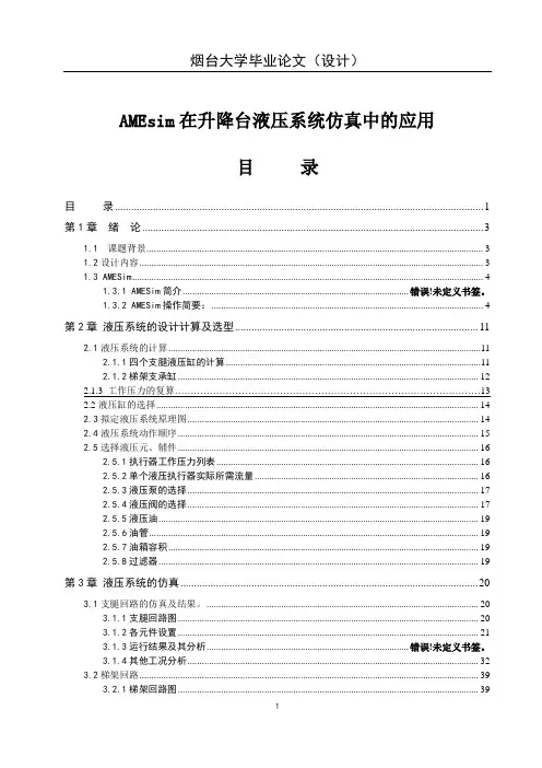
AMEsim在升降台液压系统仿真中的应用目录目录 (1)第1章绪论 (3)1.1 课题背景 (3)1.2设计内容 (3)1.3 AMESim (4)1.3.1 AMESim简介........................................................................................... 错误!未定义书签。
1.3.2 AMESim操作简要: (4)第2章液压系统的设计计算及选型 (11)2.1液压系统的计算 (11)2.1.1四个支腿液压缸的计算 (11)2.1.2梯架支承缸 (12)2.1.3 工作压力的复算 (13)2.2液压缸的选择 (14)2.3拟定液压系统原理图 (14)2.4液压系统动作顺序 (15)2.5选择液压元、辅件 (16)2.5.1执行器工作压力列表 (16)2.5.2单个液压执行器实际所需流量 (16)2.5.3液压泵的选择 (17)2.5.4液压阀的选择 (17)2.5.5液压油 (19)2.5.6油管 (19)2.5.7油箱容积 (19)2.5.8过滤器 (19)第3章液压系统的仿真 (20)3.1支腿回路的仿真及结果。
(20)3.1.1支腿回路图 (20)3.1.2各元件设置 (21)3.1.3运行结果及其分析................................................................................. 错误!未定义书签。
3.1.4其他工况分析 (32)3.2梯架回路 (39)3.2.1梯架回路图 (39)3.2.2回路各元件设置 (39)3.2.3运行结果 (45)总结 (54)致谢 (55)参考文献 (56)第1章绪论1.1 课题背景现有的升降台系统,应用最多的就是以汽车作为载体的升降台,在汽车上安装梯架,梯架可以绕着固定的轴在液压缸的作用下抬升,现有的升降台是以汽车马达作为动力,定量泵提供液压油,其梯架和汽车支腿的运动是匀速的运动,到达一定高度后停止运动,下降的期间也是匀速运动,虽然运动的速度平稳,但是在液压系统的速度是恒定的,不能实现加速和减速,因而灵活性降低,效率也会受到影响,同时,在启动和换向的时候会带来刚性冲击,对液压元件的寿命也会产生影响,并且安全系数降低,鉴于此,我们在现有的液压系统中,增加一个调节速度的元件调速阀,这样就可以实现梯架在升起和降落时的速度调节,在梯架运动过程中实现速度的变化,同时在换向和启动时的刚性冲击也就变为柔性冲击,对整个液压系统的灵活性、效率和使用寿命都将是一次巨大的改进。
我大致分了一下工,一共分3分:(1)说明书(2)总装图A0+联系他,对他讲解(3)剩余的2.5张A0图纸。
本文为对AMESIM2010自带帮助文件的翻译,限于读者水平所限,翻译中有不妥的地方希望大家批评指正!1.1 引言AMESIM液压系统包括:●常用液压元件:泵、马达等●胶皮管和管路的子模型●压力源和流量源●压力和流量传感器●液体属性定义液压系统是通过控制液体流动来完成某项功能。
这意味着它需要借助别的元件库共同工作,常用的元件库如下:机械库:将液压能量传递到机械设备信号控制库:用来控制液压系统液压元件库:用来建立液压系统液压阻力库:主要包括液压弯头和连接头,主要用在冷却和润滑系统中。
注意:液压系统中可定义多种液体,这主要用在冷却和润滑系统中。
液压环境假设一个统一的温度,如果温度需要发生变化,就需要使用变温液压库。
液压库同时包含汽蚀模型和两相流模型(用在考虑气体的液压系统)。
第一章主要是设计了几个简单的实例应用,强烈建议大家学习一下这几个例子。
特别是第三章和第五章的例子,都是基础的和必须掌握的。
1.2 例1:一个简单的液压系统目标:建立一个简单的液压系统介绍最简单的管路子模型运用汽蚀理论解释实验结果图1.1 一个简单的液压系统本例子是液压系统中最简单的实例,它主要有液压库(蓝色)和机械库组成。
原动机输出动力给泵,液体带动马达转动,马达连接一旋转机械,溢流阀设置某一固定值,超过这个值就开始溢流,实际是泵站压力。
第一个文件夹包含了液压系统常用的液压组件,第二个包含了特殊的。
通过单击文件夹可以看到里面包含的元件。
拖动元件到工作区可实现对元件的应用。
图1.2 第一个液压库第一步:用新建按钮建立一个液压控制系统选择libhydr.amt点击OK就可以建立一个新的液压系统,然后一个液压的标志按钮会出现在窗口的左上角。
也可以通过新建按钮不过这样需要手动将液压按钮放到系统中。
第二步:建立液压系统并设置子模型1.建立图1.1中的液压系统。
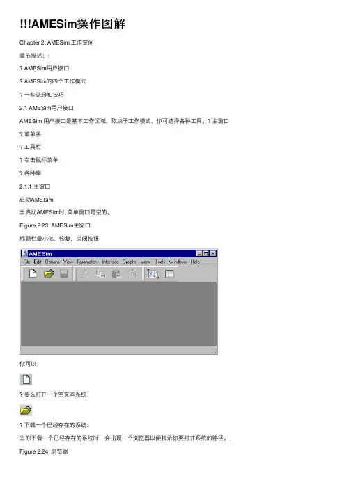
AMESim操作图解Chapter 2: AMESim ⼯作空间章节描述::AMESim⽤户接⼝AMESim的四个⼯作模式⼀些诀窍和技巧2.1 AMESim⽤户接⼝AMESim ⽤户接⼝是基本⼯作区域,取决于⼯作模式,你可选择各种⼯具。
? 主窗⼝菜单条⼯具栏右击⿏标菜单各种库2.1.1 主窗⼝启动AMESim当启动AMESim时, 菜单窗⼝是空的。
Figure 2.23: AMESim主窗⼝标题栏最⼩化,恢复,关闭按钮你可以:要么打开⼀个空⽂本系统:下载⼀个已经存在的系统:当你下载⼀个已经存在的系统时,会出现⼀个浏览器以便指⽰你要打开系统的路径。
. Figure 2.24: 浏览器1. 选择你要打开的系统并点击打开项“Open”,2. 或者双击要打开的系统。
关闭AMESim当你关闭主窗⼝时,就⾃动退出了AMESim。
要关闭主窗⼝,按如下即可:点击关闭按忸(close),按Ctrl+Q键,在主菜单中选择⽂件菜单中退出键(File _ Quit),我们将描述AMESim W主接⼝的组成(请参见图表2.23)2.1.2 主菜单主菜单使你进⼊AMESim的主特征。
Figure 2.25: 主菜单注:通过菜单中已经给出的键盘快捷键还有其它⼀些特征,请参见键盘快捷键列表。
2.1.3 ⼯具栏⼯具栏显⽰了对应于AMESim主特征的按钮。
你可以选择好多种⼯具栏:在所有模式下:⽂件操作⼯具栏模型操作⼯具栏注释⼯具栏瞬时分析⼯具栏在运⾏模式下:后台处理⼯具栏线性分析⼯具栏要了解AMESim更多的⼯作模式,请见34页“AMESim的四个⼯作模式”。
⽂件操作⼯具栏要创建草图,请打开新系统。
要修改或完成已经存在的系统请打开它。
保存你创建系统。
模式操作⼯具栏Figure 2.26: 草图模式Figure 2.27: ⼦模型模式Figure 2.28: 参数模式Figure 2.29: 运⾏模式模式操作⼯具栏依你正在⼯作的模式⽽改变。
我大致分了一下工,一共分3分:(1)说明书(2)总装图A0+联系他,对他讲解(3)剩余的2.5张A0图纸。
本文为对AMESIM2010自带帮助文件的翻译,限于读者水平所限,翻译中有不妥的地方希望大家批评指正!1.1 引言AMESIM液压系统包括:●常用液压元件:泵、马达等●胶皮管和管路的子模型●压力源和流量源●压力和流量传感器●液体属性定义液压系统是通过控制液体流动来完成某项功能。
这意味着它需要借助别的元件库共同工作,常用的元件库如下:机械库:将液压能量传递到机械设备信号控制库:用来控制液压系统液压元件库:用来建立液压系统液压阻力库:主要包括液压弯头和连接头,主要用在冷却和润滑系统中。
注意:液压系统中可定义多种液体,这主要用在冷却和润滑系统中。
液压环境假设一个统一的温度,如果温度需要发生变化,就需要使用变温液压库。
液压库同时包含汽蚀模型和两相流模型(用在考虑气体的液压系统)。
第一章主要是设计了几个简单的实例应用,强烈建议大家学习一下这几个例子。
特别是第三章和第五章的例子,都是基础的和必须掌握的。
1.2 例1:一个简单的液压系统目标:建立一个简单的液压系统介绍最简单的管路子模型运用汽蚀理论解释实验结果图1.1 一个简单的液压系统本例子是液压系统中最简单的实例,它主要有液压库(蓝色)和机械库组成。
原动机输出动力给泵,液体带动马达转动,马达连接一旋转机械,溢流阀设置某一固定值,超过这个值就开始溢流,实际是泵站压力。
第一个文件夹包含了液压系统常用的液压组件,第二个包含了特殊的。
通过单击文件夹可以看到里面包含的元件。
拖动元件到工作区可实现对元件的应用。
图1.2 第一个液压库第一步:用新建按钮建立一个液压控制系统选择libhydr.amt点击OK就可以建立一个新的液压系统,然后一个液压的标志按钮会出现在窗口的左上角。
也可以通过新建按钮不过这样需要手动将液压按钮放到系统中。
第二步:建立液压系统并设置子模型1.建立图1.1中的液压系统。
基于AMEsim的液压系统建模与仿真AMEsim是一款基于物理原理的立体化多领域建模仿真软件,在液压系统的建模和动态仿真方面拥有丰富的经验和成果,可以充分应用于液压系统仿真与分析。
本文将介绍基于AMEsim的液压系统建模与仿真方法。
1.液压系统的建模方法液压系统可分为三个主要部分:液压源、执行机构和控制系统。
在液压系统的建模过程中,分别对三个部分进行建模,并将它们组合起来形成完整的系统模型。
主要步骤如下:(1)液压源的建模:将液压源转化为不同类型的源模型,如稳态源、瞬态源、压力源等。
液压源的模型主要根据实际情况来确定,一般情况下可以使用采用数据拟合方法获取的源模型参数。
(2)执行机构的建模:执行机构包括缸、阀、单向阀、液压马达等。
执行机构的建模是基于其二阶系统的性质进行的。
液压元件可以使用自带元件库中的模型,也可以根据实际情况自行编写模型。
(3)控制系统的建模:控制系统的模型包括控制器、信号传递元件等。
控制器的建模可以使用PID控制器等自带控制器的模型,也可以根据实际情况自行编写控制器模型。
(4)系统的组合:将不同类型的源、执行机构、控制器等组合起来,形成原始系统模型。
在组合时需要考虑系统的物理连续性和能量守恒原理。
2.系统的仿真与分析方法(1)系统结构分析:对于大型液压系统,需要对其结构进行分析,确定系统中各个组件的连接方式和数量,以便给出合理的系统建模方案。
结构分析中常常采用流程图来表示各衔接部件之间的关系。
通过系统结构分析可了解系统的工作原理和特点,为系统建模和仿真提供较为明确的方向和指导。
(2)参数优化分析:参数优化分析是液压系统优化设计的重要环节。
通过参数优化可以获得液压系统的运行参数,如压力、流量、功率等,可以根据要求进行调整和优化,以提高系统的效率和质量。
参数优化分析需要重点注意系统的控制方式、工作温度、结构特点、运动状态等因素,以便得到合理的分析结果。
(3)工况分析:对于实际应用的液压系统,需要进行不同工况下的动态仿真分析。
AMESim液压手册1.1 介绍AMESim液压手册包括:*通常组成的元件包括泵,马达,孔口,以及其他,也包括特别的阀门*小管和软管的子模型*压力和流动比率的源头*压力和流动比率的检测计*流体种类的组成压力系统孤独的存在完全是没用的,它离不开流体和过程控制。
这意味着手册必须能和其他AMESim手册相兼容。
以下的手册是经常和压力手册一起并用:机械手册应用于流体压力装置当水压能量转化为机械能量信号,控制,检测手册应用于控制和水压系统水压元件设计手册从非常基本的液压和机械单元应用于建造特别的的元件液压组成手册这是一个组成包括弯曲,丁字接头,弯头以及其他,它被用于典型的诸如冷却和润滑系统的低压装置第一节个别的案例注释*在液压手册里尽可能的用多余一种的流体,这是非常重要的因为你能够做出模型关于冷却和润滑系统的手册*液压手册假设一个统一的温度贯穿于整个系统,如果热量影响被考虑到很重要,热量液压和热量液压元件设计手册应该使用*有许多气穴和空气释放的模型在液压手册。
注释有一种特别的二相流体手册,一种典型的关于这种空气调节系统的装置第一节手册包括一系列个别的例子。
我们强烈的建议你认真的对待这些个别的例子。
这些假定你有一个基本的使用AMESim的水平。
作为一个完全最小的工作量你应该做些第三节关于AMESim手册的例子和第五节第一个关于描述如何使用一组的第一个例子1.2案例1:一个简单的液压系统目标*组建一个非常简单的液压系统*介绍一个简单的小管/软管子系统*解释一个结果使用一个特别的参考关于空气释放和空穴图形1.1 一个非常简单的液压系统在这个练习中你将要构造图形1.1中的系统,这可能是最简单具有意义的液压系统。
它是由部分液压种类(通常是蓝色)和部分机械种类元件建造液压部分由用于液压系统的标准符号组成。
主要的原动力提供泵的力量,从水槽拉动液压流体。
这种流体在压力下提供给一个驱动旋转负载液压马达,当压力达到某个值的时候一个解除阀门打开,一个马达和解除阀门的输出流回水槽,图标显示了三个水槽却非常像是仅仅一个水槽被利用了。
基于AMEsim的液压系统建模与仿真一、引言液压系统是利用液体传递能量,控制方向和力的一种传动方式。
液压系统在工业生产和机械设备中得到了广泛应用,包括汽车制造、航空航天、冶金、建筑、工程机械等领域。
而建立精准的液压系统模型并进行仿真分析对于系统设计和性能优化具有重要意义。
AMESim是一款专业的多物理领域仿真软件,具有稳定、可靠的仿真算法,能够对液压系统进行精确的建模和仿真分析。
本文将介绍基于AMESim的液压系统建模与仿真的方法,通过具体案例来展示其应用价值。
二、液压系统建模方法1. 液压元件建模在AMESim中,液压系统的建模是基于液压元件的模型。
液压元件可以分为液压源、执行元件、控制元件和辅助元件四类。
液压泵、液压缸、换向阀、节流阀等都可以在AMESim 中进行建模。
建模液压元件时,需要考虑其物理特性和动态行为,并根据实际工况和使用要求设置其参数。
在液压泵的建模中,需要考虑其排量、转速对流量和压力的影响;在液压缸的建模中,需要考虑其面积、摩擦和密封对其运动过程的影响。
液压管路在液压系统中起着传输液体、传递动力和信号的作用。
在建模时,需要考虑管路的长度、直径、摩擦、弯头、阀门等因素对液压性能的影响。
在AMESim中,可以通过设置管路的几何参数、流体介质和流动特性等来建立液压管路的模型。
通过对管路压力、流量、温度等参数的仿真分析,可以评估管路的性能和系统的稳定性。
3. 控制系统建模三、液压系统仿真分析基于AMESim的液压系统建模完成后,可以进行仿真分析以评估系统性能和优化设计。
液压系统的仿真分析主要包括以下几个方面:1. 动态特性分析通过仿真分析液压系统的动态特性,可以评估系统的响应速度、稳定性和阻尼特性等。
在动态仿真中,可以模拟系统的启动、运行和停止过程,评估系统对外部扰动的响应和抑制能力。
2. 性能优化分析通过仿真分析液压系统的性能参数,可以评估系统的功率输出、效率、热量损失、工作温度等。