AMESim_液压系统建模引发的数字挑战s
- 格式:pdf
- 大小:69.07 KB
- 文档页数:12
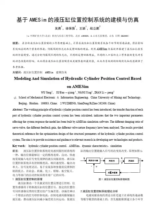
基于AMESim 的液压缸位置控制系统的建模与仿真吴勇1,徐保强1,王颖1,战立鹏2(1.中国矿业大学(北京) 机电与信息工程学院,北京 100083;2.山东五征集团,山东 日照 262300)摘要: 在分析液压缸位置控制的工作原理基础上,计算出液压缸位置控制系统各个环节的传递函数,得出影响系统响应的两个重要的参数:伺服阀的阻尼比和反馈回路的增益。
利用AMESim 仿真软件搭建了液压缸位控系统的仿真模型。
通过分析伺服阀不同的阻尼比,不同的反馈回路增益,不同的入口容积大小等参数的变化对系统动态性能的影响,从而得出液压缸位置控制系统关键参数的最优值,从而为系统的的结构优化和改进提供了参考依据。
关键词:液压缸位置控制 AMESim 建模仿真Modeling And Simulation of Hydraulic Cylinder Position Control Basedon AMESimWU Yong 1, XU Bao −qiang 1 , WANG Ying 1 , ZHAN Li −peng 2(1. School of Mechanical Electronic & Information Engineering ,China University of Mining and Technology ,Beijing ,Haidian ,100083, China; 2.WUZHENG, ShanDong RiZhao 262300, China)Abstrac t : The working principle of hydraulic cylinder position control has been introduced, the transfer function of each part of hydraulic cylinder position control system has been calculated, indicates that the two important parameters affecting the system response the model has been built by AMESim simulation software. The different damping ratio of servo-valve, the different feedback gain, the different valve nature frequency have been analyzed. The results provided theoretical reference for the optimization design of the structural parameters of the hydraulic cylinder position control system. The aim is to provide assistance and guidance to relevant research in developing new technologies and products. Key words: hydraulic cylinder position control ,AMESim ,dynamic characteristics ,simulation 前言: 液压缸位置控制系统是电液伺服控制系统的一种,输出位移能够以一定的精度连续、自动、快速地复现输入电信号变化规律的液压伺服系统。
《基于AMESim的液压系统建模与仿真技术研究》篇一一、引言随着现代工业技术的不断发展,液压系统在各种机械设备中扮演着至关重要的角色。
为了更好地理解液压系统的性能,优化其设计,以及进行故障诊断和预测,建模与仿真技术显得尤为重要。
本文将介绍基于AMESim的液压系统建模与仿真技术研究,以期为相关领域的研发和应用提供有益的参考。
二、AMESim软件概述AMESim是一款功能强大的工程仿真软件,广泛应用于机械、液压、控制等多个领域。
它提供了一种直观的图形化建模环境,用户可以通过简单的拖拽和连接元件来构建复杂的系统模型。
此外,AMESim还支持多种物理领域的仿真分析,包括液压、气动、热力等。
三、液压系统建模在AMESim中,液压系统的建模主要包括以下几个方面:1. 液压元件建模:包括液压泵、液压马达、油缸、阀等元件的建模。
这些元件的模型可以根据实际需求进行参数设置和调整。
2. 流体属性设置:根据液压系统的实际工作情况,设置流体的属性,如密度、粘度等。
3. 系统拓扑结构构建:根据实际系统的结构,搭建系统拓扑结构,并设置各元件之间的连接关系。
4. 仿真参数设置:根据仿真需求,设置仿真时间、步长等参数。
四、液压系统仿真在完成液压系统的建模后,可以通过AMESim进行仿真分析。
仿真过程主要包括以下几个方面:1. 初始条件设置:设置系统的初始状态,如初始压力、流量等。
2. 仿真运行:根据设置的仿真时间和步长,运行仿真程序。
3. 结果分析:通过AMESim提供的可视化工具,分析仿真结果,如压力、流量、温度等参数的变化情况。
五、技术应用与优势基于AMESim的液压系统建模与仿真技术具有以下优势:1. 高效性:通过图形化建模环境,可以快速构建复杂的液压系统模型,提高建模效率。
2. 准确性:AMESim提供了丰富的物理模型和算法,可以准确模拟液压系统的实际工作情况。
3. 灵活性:用户可以根据实际需求,灵活地调整模型参数和仿真条件,以获得更符合实际的结果。


基于AMEsim的液压系统建模与仿真液压系统是一种广泛应用于工程和工业领域的能量传输和控制系统。
基于AMEsim的液压系统建模与仿真,可以帮助工程师和设计师更好地理解和分析液压系统的行为、性能和特性。
AMEsim是一种基于物理原理的多域建模和仿真软件,它提供了强大的建模工具和仿真环境,适用于各种不同的物理领域,包括机械、电气、流体和热力学等。
对于液压系统的建模与仿真,AMEsim提供了丰富的液压元件库和功能模块,可以方便地搭建液压系统的数学模型,并进行仿真和分析。
液压系统的建模通常包括以下几个步骤:1. 确定系统的结构和组成部分:根据液压系统的实际应用和要求,确定系统的结构和组成部分,包括液压泵、油箱、液压缸、阀门等。
在AMEsim中,可以通过将液压元件从库中拖放到模型中来进行建模。
2. 定义元件的特性和参数:液压元件的特性和参数对系统的行为和性能有很大影响。
在AMEsim中,可以通过修改元件的属性和参数来定义其特性,例如液压泵的流量和压力特性,液压缸的阻尼和摩擦特性等。
3. 建立元件之间的连接关系:液压系统的各个元件之间通过管道和管路连接,通过液压介质(通常是液压油)进行能量传递和控制。
在AMEsim中,可以使用管道和管路元件来建立元件之间的连接关系,并定义流量和压力的传递特性。
4. 设置系统的初始状态和输入条件:在进行仿真前,需要设置系统的初始状态和输入条件。
可以设置初始状态下的压力和流量分布,以及输入条件下的压力和流量变化。
在AMEsim中,可以通过设置初始值和输入信号来实现。
5. 进行仿真和分析:通过对建立好的模型进行仿真,可以得到液压系统在不同工况下的行为和性能。
在AMEsim中,可以选择不同的仿真算法和求解器,进行仿真和分析。
还可以通过绘制曲线和输出结果来对系统的行为和性能进行分析和评估。

基于AMEsim的液压系统建模与仿真液压系统是工程中常见的一种动力传输系统,它通过液压传动来实现力的传递和执行机构的动作控制。
液压系统具有传动效率高、传动力矩大、动作平稳、反应灵敏等优点,因此在机械制造、航空航天、船舶、石油化工、建筑工程等领域得到了广泛应用。
为了更好地设计和优化液压系统,工程师们常常需要对液压系统进行建模与仿真分析。
AMEsim是一种基于物理的系统级建模和仿真软件,可以用来对复杂的液压系统进行建模与仿真。
它能够快速准确地模拟液压系统的动态特性,并通过仿真分析系统的运行状态、性能和参数变化对系统进行优化。
本文将介绍使用AMEsim对液压系统进行建模与仿真的步骤和方法。
一、液压系统建模1.系统结构设计在进行液压系统建模前,需要根据实际应用场景设计系统的结构和组成。
液压系统通常包括液压源、执行元件、控制元件和辅助元件等部分。
液压源一般由油箱、泵和电动机组成,用于产生液压能。
执行元件包括液压缸、液压马达等,用于产生力和运动。
控制元件包括阀门、液压控制阀等,用于控制液压系统的动作和方向。
辅助元件包括滤油器、冷却器等,用于保护和维护液压系统。
在建模时,需要将这些部分进行合理的组织和连接。
2.建立物理模型在AMEsim中,可以通过图形化界面来建立液压系统的物理模型。
首先需要选择合适的元件模型,并将其拖放到系统工作区中。
可以选择液压缸、液压马达、液压泵、油箱、阀门等元件模型。
然后通过连接线将这些元件连接在一起,形成完整的系统结构。
在建立连接时,需要考虑元件之间的流动方向和控制信号的传递。
3.设定参数和初始条件建立物理模型后,需要对各个元件的参数进行设定。
这些参数包括液压源的功率、泵的流量和压力、执行元件的有效面积和行程、控制阀的开启和关闭时间等。
还需要对系统的初始条件进行设定,如油箱中的油液初始压力和温度等。
完成系统的物理建模后,就可以进行仿真分析。
在AMEsim中,可以通过设置仿真时程和控制信号来对系统进行仿真。

基于AMEsim的液压系统建模与仿真AMEsim是一种用于液压系统建模与仿真的软件工具,它具有强大的功能和灵活的操作界面,可以有效地模拟液压系统的动态行为,并提供详细的分析和评估。
本文将介绍基于AMEsim的液压系统建模与仿真的流程和方法。
液压系统建模的第一步是创建系统的几何模型。
在AMEsim中,可以使用建模工具创建液压元件的几何形状和结构。
可以创建油箱、泵、阀门、管道等液压元件,并将它们连接起来,形成一个完整的液压系统。
接下来,需要定义液压元件的物理参数。
包括元件的尺寸、材料、摩擦系数、液压缸的活塞面积等等。
这些参数将用于计算元件的力学行为和动态特性。
然后,需要为液压系统添加控制算法。
在AMEsim中,可以使用模型库中提供的控制算法模块,或者自定义算法来实现对液压系统的控制。
可以添加PID控制器来控制液压缸的运动,或者根据输入信号改变阀门的开启程度。
完成模型的建立后,就可以进行仿真了。
在AMEsim中,可以设置仿真的时间步长、仿真时间等参数,并运行仿真模型。
仿真过程中,AMEsim会根据模型中定义的方程和控制算法计算液压系统的动态行为,并生成仿真结果。
在仿真结果中,可以得到液压系统各个液压元件的工作状态、压力变化、流量变化等信息。
通过分析这些仿真结果,可以评估液压系统的性能和优化设计。
可以分析液压系统的响应时间、能耗、泄漏等方面,以优化系统的性能。
基于AMEsim的液压系统建模与仿真是一个有效的工具,可以帮助工程师模拟和评估液压系统的动态行为。
通过建立液压系统的几何模型、定义物理参数、添加控制算法,并进行仿真分析,可以得到详细的系统工作状态和性能评估,从而指导液压系统的设计优化与改进。

基于AMEsim的液压系统建模与仿真AMEsim是一款应用较广泛的多领域仿真软件,可以用于机械、液压、电气、热力等领域的建模与仿真。
在液压系统方面,AMEsim可以建立液压系统的数学模型,并进行仿真验证,以使得系统设计更加精确和可靠。
下面我们将详细介绍如何使用AMEsim建立液压系统模型和进行仿真分析。
第一步:选择系统元件和建立元件库在建立液压系统模型之前,需要在AMEsim中选择系统所需要的元件,并按照实际的液压系统结构合理地建立元件库。
液压系统中常用的元件有液压泵、液压阀、液压缸、油液储存器、油液滤清器等。
建立元件库的过程中需要考虑元件的参数、功能、接口等因素。
第二步:建立系统模型在建立系统模型时,需要根据实际情况选择不同的模型组件。
例如,如果建立一个液压泵模型,则可以选择从库中拖出液压泵元件,并对其参数进行设置。
在这个过程中,需要注意参数设置对模型精度的影响。
对于每个模型组件,都需要精细地调整其参数和接口,以确保模型结果的准确性。
第三步:仿真验证在液压系统模型建立完成之后,可以通过模拟仿真来验证模型的可行性和准确性。
仿真操作可以模拟实际系统运动状态和参数变化,以进一步优化系统设计。
在进行仿真分析时,可以通过可视化图像和数值数据,直观地了解各个部件的运行状态和整个系统的性能。
总之,AMEsim提供了一种良好的液压系统建模与仿真平台,为我们设计高效、稳定、可靠的液压系统提供了重要支持。
在使用AMEsim进行建模和仿真分析时,应注意参数设置和建模组件的精细调校,并进行准确性和可行性验证,以保证模型结果和仿真分析的准确性和可靠性。
基于AMEsim的液压系统建模与仿真液压系统是工程中常见的一种动力传动系统,它通过液体传递能量来驱动机械设备。
液压系统具有传递功率大、传动效率高、操作简便、响应速度快等优点,被广泛应用于工程机械、航空航天、冶金采矿等领域。
在液压系统的设计和优化过程中,建模与仿真是非常重要的工具,可以帮助工程师们更好地理解系统工作原理、分析系统性能并进行优化设计。
本文将介绍基于AMESim的液压系统建模与仿真技术。
一、AMESim的基本介绍AMESim(Advanced Modeling Environment for Simulation of Engineering Systems)是由法国FDS公司研发的一种多物理仿真软件,旨在为工程师提供一个全面的仿真平台,用于分析和优化系统的动态性能。
AMESim具有图形化建模界面、丰富的预定义组件库、强大的仿真求解器等特点,可以用来建模与仿真多种工程领域的系统,包括机械、电气、液压、热力等。
二、液压系统建模与仿真1. 液压系统建模液压系统通常由液压泵、执行元件、控制阀、油箱和管路等组成,液体在其中传递能量并驱动执行机构。
在AMESim中,可以使用预定义的液压元件来建模系统的各个部分,如液压泵、液压缸、液压阀等。
通过简单的拖拽操作和连接线,可以快速构建出一个完整的液压系统模型。
2. 液压系统参数设置在建模过程中,需要为液压系统的各个组件设置参数,包括泵的流量、缸的活塞面积、阀的流量特性等。
AMESim提供了丰富的组件参数设置界面,用户可以直观地输入参数数值,并且支持参数的参数化设置,方便用户进行灵敏度分析和参数优化。
建模完成后,可以使用AMESim内置的仿真求解器对液压系统进行仿真。
用户可以设定系统的工况和输入信号,例如泵的转速、阀的开度、负载的变化等,然后进行仿真运行。
AMESim会自动求解系统的动态行为,并输出相关的性能指标,如压力、流量、速度、功率等,可以用于系统性能分析和优化设计。

基于AMEsim的液压系统建模与仿真
AMEsim是一种用于液压系统建模与仿真的工具。
液压系统是利用液体作为传动介质的系统,常见于许多工程领域,如工程机械、航空航天和汽车工业等。
液压系统的建模与仿真是在计算机上对液压系统进行模拟,以预测系统的性能和行为。
液压系统的建模与仿真主要包括以下几个步骤:建立系统几何模型、确定系统的物理特性、建立系统控制模型,并进行仿真分析。
建立系统几何模型。
通过绘制液压系统的图形,包括液压缸、液压泵、阀门等组件的位置和连接关系,确定系统的结构和布局。
这一步骤的目的是为了在仿真中准确地表示系统的几何形状。
确定系统的物理特性。
液压系统涉及许多物理参数,如液压缸的内径、杆径、活塞行程等,液压泵的流量和压力等。
这些参数对系统的性能和行为有重要影响,需要在建模过程中进行准确的设定。
可以通过实验或者产品手册获得这些参数。
然后,建立系统控制模型。
液压系统的控制是通过调节阀门来实现的,阀门的开度和位置会影响液压系统的压力、流量等。
在建立系统控制模型时,需要考虑阀门的特性曲线和控制策略,并根据实际情况进行设定。
进行仿真分析。
利用AMEsim提供的仿真功能,输入系统的几何模型、物理特性和控制模型,进行仿真计算。
通过仿真,可以观察系统的动态响应和性能指标,如工作压力、液压油温、流量等。
还可以对系统进行优化和改进,以实现更好的性能和效果。

基于AMEsim的液压系统建模与仿真AMEsim是一种面向物理系统的仿真软件,也可以用于液压系统的建模与仿真。
液压系统是一种运用液体传递能量来实现动力传递和控制的系统,由于其具有高功率、高工作压力和大承载能力等优点,被广泛应用于工业和机械领域。
液压系统建模与仿真是通过建立系统的数学模型,分析系统的动态特性和稳态性能,以便于优化设计和性能预测。
AMEsim提供了一种直观的建模与仿真环境,可以方便地进行液压系统的建模和仿真。
在液压系统的建模过程中,首先要确定系统的结构和组成部分。
液压系统由液压泵、执行器、阀门、油箱等组成,每个组成部分都有特定的功能和参数。
在AMEsim中,可以通过选择和配置对应的组件模型,构建系统的整体结构,并对组件进行参数设置。
接下来,需要建立系统的数学模型。
液压系统是基于流体力学原理的动态系统,主要包括质量守恒、能量守恒和动量守恒等方程。
在AMEsim中,可以通过连接各个组件,建立液压系统的动态方程。
可以设置初始条件和外部输入,以模拟真实工况下的系统性能。
然后,可以进行系统的仿真分析。
AMEsim提供了丰富的模型库和仿真工具,可以对系统的运动性能、力学特性和能量转换进行仿真分析。
可以通过仿真结果,评估系统的性能,并进行设计优化。
AMEsim还支持多种分析方法,如频域分析、鲁棒性分析和故障诊断等,可以更全面地评估系统的可靠性和稳定性。
可以通过仿真结果进行系统的验证和验证。
通过与实际实验结果进行比较,可以检查和验证建模的准确性。
如果模型与实际结果存在偏差,可以进行参数调整和改进模型,直到满足设计要求。
液压/机械系统的建模、仿真及动力学分析软件AMESim介绍AMESim 软件介绍AMESim 为流体动力(流体及气体)、机械、热流体和控制系统提供一个完善、优越的仿真环境及最灵活的解决方案。
AMESim使用户能够借助其友好的、面向实际应用的方案,研究任何元件或回路的动力学特性。
这可通过模型库的概念来实现,而模型库可通过客户化不断升级和改进。
基本特性设计框架作为设计软件包,AMESim为用户提供了一个完善的时域仿真(包括线性分析及各种专业特性)建模环境。
工程师可使用已有模型和(或)建立新的子模型元件,来构建优化设计所需的实际原型。
用户界面易于识别的标准ISO图标和简单直观的多端口框图,为用户提供了一个友好的界面,方便用户建立复杂系统及用户所需的特定应用实例。
求解器-算法自适应和强大的不连续性处理能力基于最先进的数字积分器, AMESim求解器根据系统的动态特性,在17种可选算法中自动选择最佳积分算法,并具有精确的不连续性处理能力,正是AMESim这些独创的技术,保证了仿真的速度和精度。
应用库12个开放的模型库基于物理原理和实际应用,包含大量一维流体/机械系统设计及仿真所必需的模型。
用户无须是仿真专家,轻易便可获得最新专业技巧。
超元件功能超元件功能使用户可以将一组元件集成为一个超元件,后者可以象普通元件一样使用。
由于多端口方案等原因, AMESim的超元件功能与其它软件的相应特性具有本质的差别。
开放性内置与C (或Fortran)和其它系统仿真软件的接口。
借助此特性,用户可以在AMESim环境中访问任何C 或Fortran 程序、控制器设计特征、优化工具及能谱分析等工具。
同时用户还可以将一个完全非线性AMESim子模型输出到一个CAE或多体软件中去。
AMESet 子模型编辑工具借助于AMESet,用户可以自己开发标准的、可重复使用的、便于维护的、并附有完整文档的模型库。
模型库标准库:机械- 控制可选:液压- 液压管路- 液压元件设计(即原来的AMEBel)- 液压阻力- 气动- 热- 热流体- 冷却- 动力传动- 填注。
基于AMEsim的液压系统建模与仿真AMEsim是一款基于物理原理的立体化多领域建模仿真软件,在液压系统的建模和动态仿真方面拥有丰富的经验和成果,可以充分应用于液压系统仿真与分析。
本文将介绍基于AMEsim的液压系统建模与仿真方法。
1.液压系统的建模方法液压系统可分为三个主要部分:液压源、执行机构和控制系统。
在液压系统的建模过程中,分别对三个部分进行建模,并将它们组合起来形成完整的系统模型。
主要步骤如下:(1)液压源的建模:将液压源转化为不同类型的源模型,如稳态源、瞬态源、压力源等。
液压源的模型主要根据实际情况来确定,一般情况下可以使用采用数据拟合方法获取的源模型参数。
(2)执行机构的建模:执行机构包括缸、阀、单向阀、液压马达等。
执行机构的建模是基于其二阶系统的性质进行的。
液压元件可以使用自带元件库中的模型,也可以根据实际情况自行编写模型。
(3)控制系统的建模:控制系统的模型包括控制器、信号传递元件等。
控制器的建模可以使用PID控制器等自带控制器的模型,也可以根据实际情况自行编写控制器模型。
(4)系统的组合:将不同类型的源、执行机构、控制器等组合起来,形成原始系统模型。
在组合时需要考虑系统的物理连续性和能量守恒原理。
2.系统的仿真与分析方法(1)系统结构分析:对于大型液压系统,需要对其结构进行分析,确定系统中各个组件的连接方式和数量,以便给出合理的系统建模方案。
结构分析中常常采用流程图来表示各衔接部件之间的关系。
通过系统结构分析可了解系统的工作原理和特点,为系统建模和仿真提供较为明确的方向和指导。
(2)参数优化分析:参数优化分析是液压系统优化设计的重要环节。
通过参数优化可以获得液压系统的运行参数,如压力、流量、功率等,可以根据要求进行调整和优化,以提高系统的效率和质量。
参数优化分析需要重点注意系统的控制方式、工作温度、结构特点、运动状态等因素,以便得到合理的分析结果。
(3)工况分析:对于实际应用的液压系统,需要进行不同工况下的动态仿真分析。
基于AMEsim的液压系统建模与仿真AMEsim是一种多领域建模和仿真软件,被广泛应用于液压系统的建模和仿真。
液压系统是利用液体流动和压力进行能量传递和控制的系统,包括液压传动系统、液压控制系统和液压执行机构等。
在工程领域,液压系统被广泛应用于机械、汽车、航空航天、船舶等众多领域。
在基于AMEsim的液压系统建模和仿真中,首先需要进行系统的建模工作。
液压系统的建模可以从宏观和微观两个层面进行。
在宏观层面,可以采用系统级建模方法,将整个液压系统看作一个黑箱,通过确定系统的输入和输出,建立数学模型来描述系统的动态特性。
在微观层面,可以采用元件级建模方法,将液压系统分解为各个液压元件,如液压泵、液压阀、液压缸等,并建立各个元件的数学模型。
通过这些数学模型,可以描述液压元件的运动学和动力学特性,从而揭示系统的工作原理。
液压系统的建模和仿真既涉及液压学理论的应用,也涉及数学建模和仿真技术的应用。
对于进行基于AMEsim的液压系统建模和仿真的工程师来说,既需要具备液压学理论的知识,又需要具备数学建模和仿真技术的能力。
在实际应用中,基于AMEsim的液压系统建模和仿真可以大大提高工程设计的效率和质量。
通过建立液压系统的数学模型,可以在计算机上进行仿真分析,从而可以预测和评估系统的工作性能、优化系统的设计参数、分析系统的故障和故障诊断等。
通过仿真分析,可以在设计阶段就发现问题,并进行优化设计,从而减少试制样机的制作和试验的时间和成本。
基于AMEsim的液压系统建模和仿真是一种有效的工程手段,可以在设计阶段对液压系统进行系统分析和优化设计,提高系统的可靠性、工作效率和性能。
随着计算机技术的不断发展,基于AMEsim的液压系统建模和仿真将在工程实践中得到更广泛的应用。
《基于AMESim的液压系统建模与仿真技术研究》篇一一、引言液压系统在许多工业领域中都扮演着关键的角色,其工作性能直接影响到设备的运行效率和安全性。
随着计算机技术的发展,利用仿真软件对液压系统进行建模与仿真已成为现代设计和研发的重要手段。
AMESim作为一款强大的工程仿真软件,被广泛应用于液压系统的建模与仿真。
本文旨在研究基于AMESim的液压系统建模与仿真技术,以提高液压系统的设计效率和性能。
二、AMESim软件及其在液压系统建模与仿真中的应用AMESim是一款多学科复杂系统建模与仿真软件,广泛应用于机械、液压、控制等多个领域。
在液压系统建模与仿真中,AMESim提供了丰富的液压元件模型和仿真环境,可以方便地构建各种复杂的液压系统模型。
通过AMESim,我们可以对液压系统的动态特性进行深入分析,优化系统设计,提高系统的性能和效率。
三、基于AMESim的液压系统建模基于AMESim的液压系统建模主要包括以下几个步骤:1. 确定液压系统的结构和功能。
根据实际需求,确定液压系统的基本结构和需要实现的功能。
2. 选择合适的元件模型。
在AMESim中,有丰富的液压元件模型可供选择,如液压泵、液压缸、阀等。
根据实际需求,选择合适的元件模型。
3. 建立液压系统模型。
在AMESim的建模环境中,根据选定的元件模型和系统结构,建立液压系统的模型。
4. 设置仿真参数。
根据实际需求,设置仿真参数,如仿真时间、步长等。
四、基于AMESim的液压系统仿真在建立好液压系统模型后,可以进行仿真分析。
AMESim提供了丰富的仿真工具和分析方法,可以对液压系统的动态特性进行深入分析。
具体步骤如下:1. 运行仿真。
在AMESim中运行仿真,观察系统的输出和性能。
2. 分析仿真结果。
根据仿真结果,分析系统的动态特性、稳定性等性能指标。
3. 优化设计。
根据分析结果,对系统设计进行优化,提高系统的性能和效率。
五、实例分析以某液压挖掘机为例,采用AMESim进行液压系统建模与仿真。
基于AMEsim的液压系统建模与仿真1. 引言1.1 研究背景深入研究基于AMEsim的液压系统建模与仿真方法具有重要意义。
通过建立高效精确的模型,优化系统参数,提高系统性能,可以为工程领域的液压系统设计与优化提供重要的理论支撑。
为此,本文将围绕AMEsim液压系统建模方法、建模步骤、仿真分析、参数优化和性能评估等方面展开深入探讨,旨在为液压系统的设计和优化提供参考依据。
1.2 研究目的研究的目的是为了探索基于AMEsim的液压系统建模与仿真方法,通过对液压系统的建模和仿真分析,进一步深入了解液压系统的工作原理和性能特点。
通过对参数优化和性能评估的研究,提高液压系统的效率和性能,为工程实践提供技术支持。
通过对实验结果的分析和未来研究方向的展望,为液压系统的发展和应用提供理论和技术参考,推动液压系统技术的进步和创新。
通过本次研究,旨在为液压系统的设计、优化和应用提供更加科学和可靠的方法和技术支持,促进液压技术的发展和应用。
1.3 研究意义液压系统在工程领域中具有重要的应用价值,它能够将液体的流动和压力转化为力和运动。
对于液压系统建模与仿真的研究意义重大。
通过建模与仿真可以帮助工程师更好地了解液压系统的工作原理和特性,从而提高系统设计的准确性和效率。
基于AMEsim的液压系统建模与仿真可以有效减少实际试错成本,提高系统设计的可靠性和稳定性。
通过参数优化和性能评估,可以进一步优化液压系统的设计,提高系统的性能和效率。
深入研究基于AMEsim的液压系统建模与仿真具有重要的理论和实际意义,对于推动液压技术的发展和应用具有积极的促进作用。
2. 正文2.1 AMEsim液压系统建模方法AMEsim液压系统建模方法是基于AMEsim软件平台的一种建模方法,它可以帮助工程师们更准确地模拟液压系统的运行情况,从而实现系统设计、优化和性能评估。
在进行液压系统建模时,首先需要选择合适的元件模型,如液压泵、液压缸、阀等,然后根据系统的实际情况对这些元件进行连接和参数设置。
基于AMEsim的液压系统建模与仿真一、引言液压系统是利用液体传递能量,控制方向和力的一种传动方式。
液压系统在工业生产和机械设备中得到了广泛应用,包括汽车制造、航空航天、冶金、建筑、工程机械等领域。
而建立精准的液压系统模型并进行仿真分析对于系统设计和性能优化具有重要意义。
AMESim是一款专业的多物理领域仿真软件,具有稳定、可靠的仿真算法,能够对液压系统进行精确的建模和仿真分析。
本文将介绍基于AMESim的液压系统建模与仿真的方法,通过具体案例来展示其应用价值。
二、液压系统建模方法1. 液压元件建模在AMESim中,液压系统的建模是基于液压元件的模型。
液压元件可以分为液压源、执行元件、控制元件和辅助元件四类。
液压泵、液压缸、换向阀、节流阀等都可以在AMESim 中进行建模。
建模液压元件时,需要考虑其物理特性和动态行为,并根据实际工况和使用要求设置其参数。
在液压泵的建模中,需要考虑其排量、转速对流量和压力的影响;在液压缸的建模中,需要考虑其面积、摩擦和密封对其运动过程的影响。
液压管路在液压系统中起着传输液体、传递动力和信号的作用。
在建模时,需要考虑管路的长度、直径、摩擦、弯头、阀门等因素对液压性能的影响。
在AMESim中,可以通过设置管路的几何参数、流体介质和流动特性等来建立液压管路的模型。
通过对管路压力、流量、温度等参数的仿真分析,可以评估管路的性能和系统的稳定性。
3. 控制系统建模三、液压系统仿真分析基于AMESim的液压系统建模完成后,可以进行仿真分析以评估系统性能和优化设计。
液压系统的仿真分析主要包括以下几个方面:1. 动态特性分析通过仿真分析液压系统的动态特性,可以评估系统的响应速度、稳定性和阻尼特性等。
在动态仿真中,可以模拟系统的启动、运行和停止过程,评估系统对外部扰动的响应和抑制能力。
2. 性能优化分析通过仿真分析液压系统的性能参数,可以评估系统的功率输出、效率、热量损失、工作温度等。
Numerical Challenges Posed by Modeling HydraulicSystemsC.W. RichardsSociété Imagine42300 ROANNE,France.Tel. +33 4 77 23 60 37Fax. +33 4 77 23 60 31Email imagine@AbstractThis paper describes the characteristics of models of hydraulic systems which make them particularly challenging for numerical integrators. Problems associated with numerical stiffness, high index differential algebraic equations, extreme non-linearities and discontinuities are described. The consequences of hydraulic sub-systems in multi-domain simulation are discussed. Finally a plea for a new generation of integrator is made.1 IntroductionThe term hydraulic system must be taken broadly to include areas such asaircraft and rocket fuel systemsvehicle fuel injection systemscooling systemslubrication systemshydraulic braking systemshydraulic power steering systemsemploying a wide variety of fluids from water to liquid hydrogen as well as classical hydraulic systems with regular 'hydraulic' oil.The author is a numerical mathematician who has been specializing in simulating hydraulic and pneumatic systems since 1978. In this time he has encountered many numerical problems. Most of these were due to old fashioned bugs in both coding and inthe underlying model. However, there have been other persistent problems which have to be attributed to the intrinsic nature of hydraulic systems. What are these special characteristic of models of hydraulic systems from a numerical point of view? Briefly the governing equations are numerically stiff, very non-linear, can have high index differential algebraic equations and are often modeled with discontinuities.It is interesting that during meetings for the Toolsys project [1], the author in conversation with designers of multi-body and electrical software has heard almost identical characteristics attributed to these domains. Does this mean that there is no significance difference between the numerical characteristics of these domains? In the following sections the author attempts to show that there is.Problems related to pneumatic systems are also mentioned briefly.2 Hydraulic systems are multi-domainA hydraulic system in isolation is singularly useless. It is necessary to do something with the hydraulic power. In practice this means moving some mechanical system. In addition it is necessary to control the hydraulic system. As a consequence even the simplest hydraulic systems will normally contain multi-body and control elements as well as hydraulic elements.In consequence the solver must to some extent have a multi-domain capability. However, the 'foreign' domain elements are normally relatively simple. In the AMESim hydraulic software produced by Imagine, much effort has been extended in tuning the integrator to hydraulic systems.3 Fluid PropertiesFundamental to the modeling of hydraulic systems are the fluid properties density, bulk modulus and viscosity. The hydraulic fluid will almost always contain air. This may be dissolved and/or free in the form of bubbles. At higher pressures the air will eventually become dissolved. At low pressure bubbles will form leading to a phenomenon known as air release. The process is relative slow (compared with cavitation) and with many systems the fraction of the air that is free can be taken to be constant.Cavitation occurs when the pressure in the hydraulic fluid reaches the saturated vapor pressure. This is a much faster process than air release. Cavitation is very important because when it occurs, extensive damage can be done. Previously it was enough forsimulation to predict that cavitation occurred. Now users ask that it be quantitatively correct --- a very demanding requirement. If cavitation is present but not at too serious a level, a company may have a strong price advantage over a competitor that has chosen to eliminate cavitation completely and a strong reliability advantage over another that has severe cavitation.Figures 1 to 3 show fluid properties of diesel fuel between 0 and 1000 bar gauge pressure. The fractional air content is 0.1 % by volume. In fig. 2, the plot of bulk modulus, the presence of the air greatly modifies the value.Figure 1 DensityFigure 2 Bulk modulusFigure 3 Absolute viscosityFigures 4 to 7 show the plots for the pressure range -1 to 0 bar gauge. The dramatic effect of cavitation is evident in all these graphs. In particular the zoomed view in fig. 7 shows how as the liquid changes to vapor the bulk modulus becomes almost zero. As the integrator negotiates this region a lot of step size reductions and Jacobian re-evaluations will be necessary.Figure 4 DensityFigure 5 Bulk modulusFigure 6 Absolute viscosityFigure 7 Bulk modulusNote that, since all normal hydraulic liquids are not chemically pure, the boiling of the liquid does not take place at a single pressure but over a range of pressures. However, this range can be very narrow giving very non-linear fluid properties. Without careful rewriting, integrators cannot deal with these conditions.4 Implicit and explicit systemsWe can normally express the governing equations for a hydraulic system either by a system of ordinary differential equations (ODEs)),(y t f dtdy =or by a system of differential algebraic equations (DAEs) of the form0,,(=dtdy y t Fwhere t is time and y is the vector of state variables. For DAEs there is an important measure known as the index of nilpotency. In simple terms we can always convert DAEs to ODEs by differentiation and manipulation. The smallest number of differentiations required is the index of nilpotency. ODEs have index 0. Normally index 1 problems are easy to solve, index 2 problems more difficult and index 3 problems very difficult. This is because the Jacobian matrices employed to solve the systems of equations become progressively more badly conditioned as the index increases. With high index problems (certainly 3 and perhaps 2) it is not a good idea to employ very small integration steps.As will be shown in the next section, hydraulic system governing equations can be very stiff. This means that during the initial transient behavior, very small integration steps must be used. If there is also a high index, there is a natural conflict and failure is possible.At Imagine, where the AMESim fluid power software is produced, modelers take a pride in reducing the number of DAEs used to a minimum. Other AMESim users show no such restraint and the DAE solver DASSL is used almost all the time.For a discussion of nilpotency and the DASSL integrator see reference [2].5 Hydraulic systems as electrical circuitsIt is very easy to see the analogy between hydraulic systems and electrical systems. Engineering courses often stress this point. It is not surprising, therefore, to see attempts to deal with modeling and simulation of the two domains in the same way. Pressure is the same as voltage and flow rate the same as current. However, problems arise very quickly with this approach.When we join two hydraulic components we use a pipe or hose. The walls of this will expand with pressure (especially hoses) and the fluid has some compressibility (especially if it contains significant quantities of air). The most commonly used equation in hydraulic modeling is probablyV Q B dt dP ∑= 1where the time derivative of pressure is expressed in terms of the effective bulk modulus B, the volume V and the sum of the inflow Q . This equation is often used to model the compressibility effects in the pipe. Since B for a hydraulic fluid is of the order 91017x Pa, a very small time constant is introduced and the equations are numerically very stiff.In contrast we join electrical components by a wire. There is very little compressibility which is like saying B in equation 1 is infinity. Hence we use∑=0i2 This is a constraint equation whereas 1 is an ODE.Figure 8 Electrical system in AMESimFigure 8 shows an electrical system modeled using AMESim. (Some AMESim users do simulate electrical systems using AMESim.) By performing a linearization it is possible to compute the index of nilpotency which turns out to be 1.The hydraulic equivalent of equation 2 is∑=0Q 3This can be thought of as a pipe in which the effective bulk modulus is infinity or the volume is zero. This model is not without merit as using equation 1 with a very large value of B/V can give very slow simulation whereas switching to equation 3 speeds things up. Figure 9 shows an injection system in which there is a small volume, called the sac and indicated by V in the figure, next to the actual injection holes. It can be useful to model this using equation 3 resulting in faster simulation. The equations are index 2.Figure 9This model has been used internally at Imagine but has never been released as a standard AMESim model because it gets into big trouble when cavitation occurs. The problem is not just that it is index 2. Other index 2 problems are solved with contemptuous ease. The problem is that other factors are involved.If we determine a voltage V such that such that equation 2 is satisfied, there are no special restrictions on the voltage. Before convergence is obtained on an integration step, V may gets some quite extreme values. As long as convergence is obtained in the end, this is not a problem.In contrast if a pressure P is obtained using equation 3, there are fundamental restrictions on the values that P may have. We cannot have a pressure less that 0 absolute. Thus we have a combination ofan index 2 problem for which a very small step size is not a good idea;severe non-linearities in the fluid properties due to cavitation tending to reduce the integration step;restriction on the admissible value of pressure.These in combination reduce the reliability of the model.Pressure ultimately is not like voltage.6 Causal and acausal modelingThere has been some interest in recent years in acausal modeling and acausal libraries of hydraulic libraries have been proposed. Unfortunately many hydraulic components are not acausal by nature. The relief valve and check valve are good examples. If all we know is that the flow rate through them is zero, we cannot compute the pressure drop across them.A acausal model tries to get over this by assuming that these valves always leak [3]. However, real units do not suffer from this incontinent behavior and hence such modeling techniques are best avoided in hydraulic systems.7 Get the physics rightOne of the most common errors in modeling hydraulic system occurs in an orifice. All good text books on hydraulic systems give the flow rate Q through the orifice in terms of the pressure drop P ∆, density ρ, cross-sectional area A and a flow coefficient flow C asρ∆P C A Q flow 2.= 4The numerical problem with this formula is that the graph of Q against P ∆ has an infinite slope at the origin. This shows up as problems when P ∆ crosses zero. If a linearization is made at the equilibrium point, very strange results are obtained.It is often true with hydraulic systems that, if you get the physics wrong, you end up with numerical problems. The solution is simple. An orifice has linear behavior when P∆ is small. By modifying the model good results can be obtained.8 DiscontinuitiesIt is very convenient to include discontinuities in models of hydraulic and associated components. Strictly speaking a discontinuity involves a jump change in the value of a state variable and we could call this a hard discontinuity. These discontinuities will normally kill an integrator unless very careful coding is employed.An example of a hard discontinuity is in the model of a hydraulic jack in which, when the piston reaches the end of its stroke, the velocity comes instantaneously to rest. This implies a perfectly inelastic collision.Models where there is a jump change in the first or second derivative of a state variable are also used in models of hydraulic components. These 'soft' discontinuities can also give problems for the integrator.Most simulation software except multi-body software now have refined methods for handling discontinuities. For a description of running a mixed hydraulic multi-body system in a multi-body software see reference [4].9 Pneumatic systemsIn some respect modeling of pneumatic systems is easier than hydraulic systems since the governing equation are less stiff. The fluid properties are also less non-linear but the restrictions on pressures described in section 5 apply equally to pneumatic systems. In addition there are similar restrictions on temperature values.It is interesting that there is an ISO 6358 standard on the modeling of pneumatic orifices. Unfortunately the model described introduces precisely the problems described in section 7.10 Domain Specific IntegratorsAs mentioned in section 2 the integrator of AMESim has been extensively tuned for solving systems models of the domain for which it was designed. This is probably true of all electrical and multi-body software.In work for the Toolsys project the author has imported and run multi-body systems within AMESim. These were developed in COMPAMM [5]. Very simple examples ran with no problems but bigger systems required much manual adjustment to run parameters. The problem was that the multi-body sub-system model contained an iterative procedure employing a Newton type method to solve iteratively non-linear equations. The incomplete convergence of these iterations was seen by the AMESim integrator as noise which lead to much reduction in the step size, re-evaluation of Jacobians and very slow simulation. Some re-tuning of the integrator lead to very fast runs. Unfortunately this new state of tune proved very unsuitable for regular hydraulic systems.Experience running hydraulic systems created in AMESim within the Adams software [4] lead to a conflict in the needs of the two domains. The multi-body sub-system needed to avoid small integration steps whereas the hydraulic sub-system needed small step sizes. In addition all hard discontinuities had to be eliminated from the hydraulic sub-system model and in particularvalves which were normally 'stepped' open had to be 'ramped' open;cavitation had to be either avoided completely or a much simpler model had tobe employed;if actuator models employed hard discontinuities due to end-stop modelingeither great care had to be taken to ensure that there was no contact with end-stops or a difficult form of end-stop modeling had to be employed;sometimes hydraulic volumes had to be increased somewhat to 'de-stiffen' theequations.11 ConclusionsThere are numerical difficulties peculiar to hydraulic systems and these impose a severe test on the solver employed in simulation software. These solver tend to be highly tuned to a specific domain and problems occur when a non-trial foreign system is imported. Tomake multi-domain a routine activity, a new generation of numerical integrators need to be developed capable of coping efficiently with multi-body, hydraulic, pneumatic, electrical and electronic sub-systems.Development of these new range of integrators is a real challenge. If this task is left to the software suppliers, a lot of state of the art numerical analysis may be lost. If it is done by specialist numerical analysts working in universities or research institutes, contact with real industrial problems may be lost. The author believes that the best solution is for specialist numerical analysts to work very close with the simulation software suppliers.12 References[1] Toolsys, Open Toolset For Mixed Simulation of Multi-domain Systems, BRITE-EURAM Project CEC Ref No: BRPR CT96 0303[2] Brenan K.E., S.L. Campbell and L.R. Petzold, Numerical Solution of Initial-value Problems in Differential-Algebraic Equations, North Holland, 1989[3] Beater P., Object-orientated Modeling and Simulation of Hydraulic Drives, Simulation News Europe, No. 22, March 1998[4] Jansson A.J., M. Yahiaoui and C.W. Richards, Running Combined Multi-Body Hydraulic System Simulations within Adams, Proceedings of International Adams User Conference, Ann Arbor, July 1998[5] COMP uter A nalysis of M achines and M echanisms, Centro de Estudios e Investigaciones Técnicas, San Sebastian, Spain.。